How to choose a classification threshold from error costs (scikit-learn TunedThresholdClassifierCV)
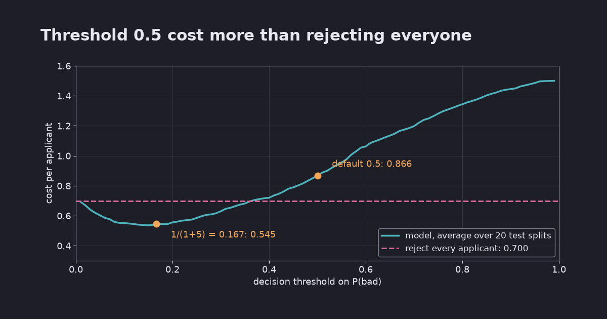
On the German Credit data, a logistic regression at the default 0.5 threshold cost 0.866 per applicant, more than rejecting everyone (0.700). The threshold from the cost matrix, 1/6, cut it to 0.545, and TunedThresholdClassifierCV found the same from training data alone. Tuning on the test set looked better than it was.
A classifier’s predict turns a probability into a yes or no at 0.5. That threshold is only right when both kinds of mistake cost the same. On a credit dataset where approving a bad applicant costs five times as much as rejecting a good one, the default threshold did worse than a rule that rejects every applicant:
| Strategy | Cost per applicant | Bad applicants caught | Good applicants rejected |
|---|---|---|---|
| Default threshold 0.5 | 0.866 | 48% | 13% |
| Reject every applicant | 0.700 | 100% | 100% |
| Threshold from the costs, 1/(1+5) = 0.167 | 0.545 | 86% | 48% |
TunedThresholdClassifierCV | 0.547 | 89% | 55% |
| Threshold tuned on the test set (a leak) | 0.507 |
All numbers are averages over 20 random 70/30 train/test splits. The model never changed; only the threshold did.
Tested on 2026-10-23 with scikit-learn 1.9.1, pandas 3.0.6 and Python 3.12.13 on Apple Silicon (macOS). Full script: threshold.py, output: threshold_out.txt. Two runs printed identical values.
The data and the costs
The Statlog German Credit dataset (Hofmann, 1994, UCI, CC BY 4.0) has 1,000 loan applicants, 30% of them labelled as bad credit risks. It is unusual because it ships with a cost matrix:
| Predicted good | Predicted bad | |
|---|---|---|
| Actually good | 0 | 1 |
| Actually bad | 5 | 0 |
So the score to minimise is the cost per applicant: (5 × bad approved + 1 × good rejected) / applicants. The positive class is “bad”, and the model is a plain pipeline: one-hot encoding, scaling and LogisticRegression.
This is a demo of the cost matrix, not a lending model. Two columns, sex/marital status and foreign-worker status, are left out of the features. A real credit model has legal and fairness requirements that this post does not cover.
Why 0.5 fails here
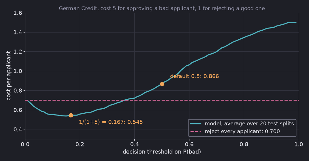
At 0.5, the model approves anyone it thinks is more likely good than bad. It caught only 48% of the bad applicants, and each one it missed cost 5. Rejecting everyone costs exactly 0.700 (the 70% who are good, times 1), and the default threshold is above that line.
The curve also shows the general shape: very low thresholds reject almost everyone, very high ones approve almost everyone (1.5 at 0.99, the 30% bad times 5), and the minimum sits where the two costs balance.
Option 1: compute the threshold from the costs
If the predicted probabilities are calibrated, you can work out the threshold directly. Reject when the expected cost of approving is higher than the expected cost of rejecting:
p × 5 > (1 − p) × 1 → p > 1 / (1 + 5) = 0.167
In general the threshold is cost_FP / (cost_FP + cost_FN). scikit-learn’s FixedThresholdClassifier applies a fixed threshold to any classifier, so the rest of your code can keep calling predict:
from sklearn.model_selection import FixedThresholdClassifier

clf = FixedThresholdClassifier(model(), threshold=1 / 6).fit(X_train, y_train)
clf.predict(X_test)   # 1 (bad) when P(bad) >= 0.167
This gave 0.545. The catch is the “if”: logistic regression is usually reasonably calibrated, but many models are not, and then the formula points at the wrong place.
Option 2: let cross-validation find it
TunedThresholdClassifierCV (added in scikit-learn 1.5) does not rely on calibration. It splits the training data, fits the model, scores many candidate thresholds with your metric on the held-out folds, and keeps the best one. The metric here is the cost, wrapped with make_scorer:
from sklearn.metrics import confusion_matrix, make_scorer
from sklearn.model_selection import TunedThresholdClassifierCV

def cost_per_applicant(y_true, y_pred):
    tn, fp, fn, tp = confusion_matrix(y_true, y_pred, labels=[0, 1]).ravel()
    return (5 * fn + 1 * fp) / len(y_true)

cost_scorer = make_scorer(cost_per_applicant, greater_is_better=False)
tuned = TunedThresholdClassifierCV(model(), scoring=cost_scorer, cv=5).fit(X_train, y_train)
tuned.best_threshold_   # between 0.090 and 0.191 across the 20 splits, 0.138 on average
It reached 0.547, the same as the formula within noise, without being told anything about calibration. By default it refits the model on all the training data afterwards. Its default scoring is balanced accuracy, so pass your own metric when your costs are not symmetric.
The trap: tuning the threshold on the test set
The tempting shortcut is to fit the model, then try thresholds on the test set and keep the best. That reported 0.507, lower than either honest method. It is not a better threshold; it is the test labels leaking into a decision. The chosen threshold jumped between 0.07 and 0.25 from split to split, because with 300 test applicants a handful of borderline cases decides where the minimum lands. Picking that minimum and reporting its cost is optimistic by construction, the same mistake as fitting preprocessing on the test data.
What to use
- Write down the costs first. If you cannot say what each kind of mistake costs, you do not know what 0.5 is optimising either. Rough numbers are better than an implicit 1:1.
- Calibrated model and clear costs: compute
cost_FP / (cost_FP + cost_FN)and useFixedThresholdClassifier. - Otherwise:
TunedThresholdClassifierCVwith a scorer for your actual metric. It also works for targets such as “recall of at least 90%” via a custom scorer. - Keep the test set out of it. Choose the threshold on training data or a validation set, then report the test result once.
- Compare with trivial rules. “Reject everyone” was a cheap baseline here and the default model lost to it; see why you should always build a baseline first.
Limits of this test
One small dataset (1,000 rows), one model, one cost matrix. With 300 test applicants per split, single-split costs ranged widely (0.740 to 0.990 at the default threshold), which is why the tables show averages over 20 splits. UCI’s newer South German Credit entry says this dataset’s coding information (which value means what) contains severe errors. That does not affect a cost-threshold demo, but do not read the coefficients as facts about borrowers. The chart comes from threshold_charts.py.
Related: Why is 99% accuracy useless? Precision, recall and F1 explained