Recursive vs direct multi-step forecasting: what a one-step score hides

26 Oct 2026 in Machine Learning & Engineering

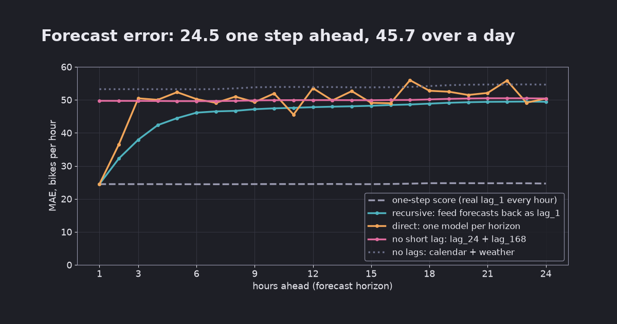
A model with lag features scored MAE 24.5 one hour ahead. Forecasting the next 24 hours, the same model averaged 45.7. Recursive, direct and “no short lag” strategies compared on real hourly data with scikit-learn, with code.

In the KFold vs TimeSeriesSplit post, a gradient-boosting model with lag features scored an MAE of 24.6 bikes per hour on the 8 weeks after its training data. That number came with a caveat: every prediction used the real demand of the previous hour. It measured predicting the next hour, not forecasting a day.

This post measures the day. From every hour in the same 8 weeks, each strategy forecasts the next 24 hours:

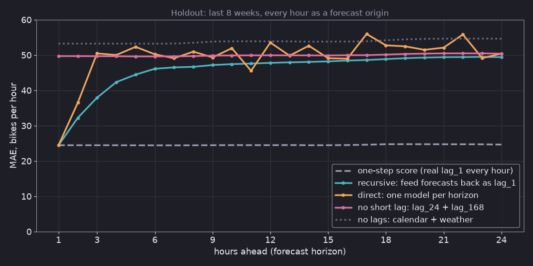
• The one-step score stays at 24.5 for every horizon, because it keeps using real values it would not have.
• A real recursive forecast starts at 24.5 one hour ahead, reaches 46.1 six hours ahead and 49.4 a day ahead, for an average of 45.7 over the 24 hours.
• Direct forecasting (one model per horizon) averaged 49.4, jumped around between neighbouring horizons and cost 24 model fits.
• A single model that simply leaves out the 1-hour lag averaged 50.0 with no recursion at all.

Tested on 2026-10-23 with scikit-learn 1.9.1, pandas 3.0.6, NumPy 2.5.4 and Python 3.12.13 on Apple Silicon (macOS). All numbers come from multistep.py (full output); repeated runs printed identical MAE values.

The setup

Same data and model as the previous post: the UCI Bike Sharing dataset (Fanaee-T, 2013, CC BY 4.0), hourly, loaded from OpenML as Bike_Sharing_Demand version 2, and HistGradientBoostingRegressor(random_state=0). The last 1,344 rows (8 weeks) are the test period; the 15,867 rows before them are for training. Features are calendar and weather columns, a row index t, and lags of the target: lag_1, lag_24 and lag_168 are the demand 1, 24 and 168 rows earlier.

Each of the 1,321 hours from the end of training to one day before the end of the data is a forecast origin: the last hour whose demand is known. Every strategy predicts the 24 rows after it, and the MAE is computed separately for each horizon h = 1 to 24. (The one-step score is 24.5 here instead of 24.6 because the last 23 hours of the data have no full 24-hour window after them and are not origins.)

Two simplifications apply to every strategy alike:

• Weather is the actual weather, not a forecast of it. A deployed model would get weather forecasts, so all the errors below are optimistic.
• A row is usually, but not always, one hour. The data skips a few hours, so “24 rows ahead” is a day ahead in most cases. The previous post measured how often (lag_1 is exactly one hour back in 99.6% of rows).

Only lag_1 needs special handling. For a target hour up to 24 rows ahead, lag_24 (the same hour yesterday) and lag_168 (the same hour last week) are already observed at the origin.

Recursive: feed forecasts back as inputs

Train one one-step model, then walk forward. For h = 1, lag_1 is the real demand at the origin. For h = 2, there is no real value yet, so lag_1 becomes the model’s own forecast for h = 1, and so on:

one_step = model().fit(X1_train, y_train)            # features: calendar, weather, t, lag_1, lag_24, lag_168
rec = np.empty((len(origins), 24))
for h in range(1, 25):
    feats = X1.iloc[origins + h].copy()               # lag_24 and lag_168 are real values for h <= 24
    if h > 1:
        feats["lag_1"] = rec[:, h - 2]                # the forecast one step earlier replaces the real value
    rec[:, h - 1] = one_step.predict(feats)

All 1,321 origins are predicted together, one horizon at a time, so this takes 24 predict calls, not 31,704.

Direct: one model per horizon

Instead of guessing lag_1, train a separate model for each horizon h. Model h uses lag_h: the demand h rows before the target, which is exactly the last value known at the origin. Model 1 is the one-step model again; model 24 has only lag_24 and lag_168.

for h in range(1, 25):
    Xh = with_lags(X, y, sorted({h, 24, 168}))        # lag_h replaces lag_1
    direct[:, h - 1] = model().fit(Xh.iloc[train], y[train]).predict(Xh.iloc[origins + h])

The third strategy is the simplest: one model with lag_24 and lag_168 only. It needs no recursion, because no input is ever in the future, but it gives up the most recent hour.

The results

Strategy	h=1	h=2	h=3	h=6	h=12	h=24	Mean, 1-24
One-step score (real lag_1 every hour)	24.5	24.5	24.5	24.4	24.5	24.6	24.5
Recursive	24.5	32.2	37.9	46.1	47.8	49.4	45.7
Direct (24 models)	24.5	36.5	50.5	50.2	53.5	50.4	49.4
lag_24 + lag_168 only	49.7	49.7	49.7	49.6	49.9	50.4	50.0
No lags (calendar + weather)	53.2	53.2	53.2	53.2	53.9	54.6	53.9

The one-step score is not a day-ahead number. It stays flat because it never runs out of real inputs. A real forecast for the next 24 hours averaged 45.7 in the best case here, almost twice as high. If you report the first number for a system that plans a day ahead, you report half the error.

The 1-hour lag helps for a few hours, then fades. Recursive is clearly better than the no-short-lag model for the first hours (32.2 vs 49.7 at h = 2), and the gap shrinks to 3.5 at h = 6 and 1.0 at h = 24. Errors compound because each step feeds on the previous forecast, but here they did not run away: the recursive curve levels off just below the no-short-lag model, which is the information it falls back to.

Direct was the least stable. In theory, direct forecasting avoids compounding errors because no model ever sees its own forecasts. Here, after the first two hours, the per-horizon models were worse than the single lag_24 model at 14 of 22 horizons. Their MAE ranged from 45.5 (h = 11) to 56.0 (h = 17), with jumps of up to 8 between neighbouring horizons. Each model is a separate fit, so each one carries its own fitting noise. They also cost 24 fits: 7 to 12 seconds across runs here, against under half a second for one model.

Is the ranking an artefact of the model settings?

With more than 10,000 rows, HistGradientBoostingRegressor turns on early stopping by default and sets aside a random 10% of the training rows to monitor it. To check that this did not decide the comparison, the script runs every strategy again with early_stopping=False, training on all rows:

Strategy	Mean MAE, default	Mean MAE, early_stopping=False
One-step score	24.5	24.0
Recursive	45.7	44.8
Direct	49.4	47.0
lag_24 + lag_168 only	50.0	45.9
No lags	53.9	50.7

All numbers moved, by up to 4 bikes per hour, so treat differences of one or two as noise. The pattern held: recursive had the lowest average, the one-step score was still about half of it, and direct still jumped between horizons (from 45.8 to 52.4 after h = 2). The model without a short lag came within 1.1 of recursive, and was slightly better at the far end (46.4 vs 47.5 at h = 24).

What to use

• Evaluate at the horizon you deploy. If the system plans tomorrow at midnight, score forecasts made at midnight for the next 24 hours, with only the values available at midnight. Report the error per horizon, not just one number.
• Start with recursive or with “only lags you will have”. Both are one model. Recursive used the latest observation best in the first hours; dropping lags shorter than the horizon was almost as good over a full day and has no feedback loop to debug.
• Try direct when you have a reason, such as a horizon-specific pattern or a model that is badly biased when fed its own forecasts, and check the per-horizon curve for jumps. On this data it was the most expensive and the least stable option.
• Keep the weather caveat in mind. Real day-ahead forecasts get forecast weather, so expect higher errors than any number here.

Limits of this test

One dataset, one model family, one 8-week period, 24-hour horizons, and actual instead of forecast weather. The size of each gap will be different on your data; the parts to expect elsewhere are the gap between the one-step score and a real multi-step forecast, and the need to look at error per horizon. scikit-learn has no built-in multi-step forecaster; the loop above is all there is to it. Libraries such as skforecast and sktime wrap both strategies, but they were not used here. The charts come from multistep_charts.py.

Related: Why fit preprocessing on training data only? A data leakage demo · Why you should always build a baseline model first