Do you need a vector database? Exact search vs HNSW on 134,000 real embeddings

19 Oct 2026 in AI & Developer Tips

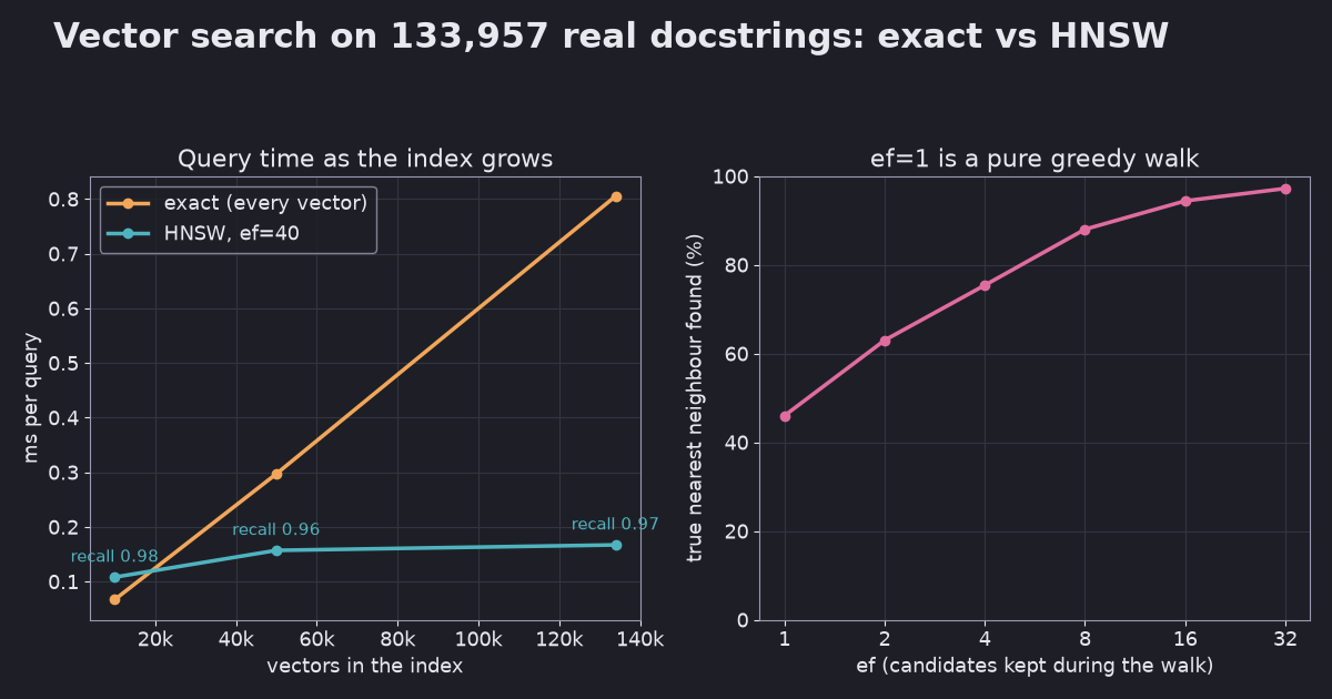
We embedded 134k docstring paragraphs with a local model and compared exact nearest-neighbour search with an HNSW index. Exact search grew from 0.07 to 0.8 ms per query; HNSW stayed near 0.17 ms at 97% recall. And with only one candidate, HNSW’s greedy walk found the true nearest neighbour less than half the time.

Semantic search turns every text into a vector and returns the vectors closest to the query (embeddings explained). The simplest way to find them is to compare the query with every vector. Vector databases use an approximate index instead, most often HNSW (Hierarchical Navigable Small World). The question is when the approximation is worth it.

We measured both on real text:

Vectors in the index	Exact search	HNSW (ef=40)	HNSW recall@10
10,000	0.067 ms	0.108 ms	0.976
50,000	0.297 ms	0.157 ms	0.962
133,957	0.805 ms	0.167 ms	0.972

Exact search grows in a straight line with the data. HNSW barely moves, but it misses about 3% of the true top-10. At 10,000 vectors, exact search was the faster one.

Tested on 2026-10-14 with Python 3.12.13, sentence-transformers 6.1.0 (all-MiniLM-L6-v2), NumPy 2.5.4 and hnswlib 0.8.0 on an Apple Silicon Mac, locally with no API key.

The data: real text, nothing to download

We needed a large set of real sentences without downloading a dataset. Every Python installation has one: the docstrings. The corpus script reads every .py file in the standard library and the installed packages with ast (nothing is imported), keeps docstring paragraphs of 40–400 characters, and embeds them with all-MiniLM-L6-v2. That gave 134,457 unique paragraphs, 384 numbers each.

500 paragraphs were held out as queries and never added to the index, so no query can find itself.

Exact search is one matrix multiplication

With normalized vectors, cosine similarity is a dot product, so exact search for a batch of queries is a single matrix multiplication followed by picking the top 10:

def exact(db, qs, k):
    scores = qs @ db.T                                   # cosine similarity: vectors are normalized
    top = np.argpartition(-scores, k, axis=1)[:, :k]
    order = np.argsort(-np.take_along_axis(scores, top, axis=1), axis=1)
    return np.take_along_axis(top, order, axis=1)

It is always correct (recall 1.0), and its cost is proportional to the number of vectors. One caveat about the timings: NumPy multiplies the 500 queries as one batch using all cores, while the HNSW queries ran on one thread. Searching one query at a time would make exact search look slower than in the table.

HNSW: a greedy walk on a graph

HNSW links every vector to a few of its neighbours, building a graph. A search starts at an entry point and keeps moving to whichever neighbour is closer to the query, until no neighbour is closer. It is the same idea as A* in our path search post: use a sense of direction to avoid looking at everything. The index has extra sparse layers on top for long jumps, which is the “hierarchical” part (Malkov and Yashunin, arXiv:1603.09320, checked 2026-10-14).

index = hnswlib.Index(space="ip", dim=db.shape[1])
index.init_index(max_elements=len(db), M=16, ef_construction=200, random_seed=100)
index.add_items(db, np.arange(len(db)))
index.set_ef(40)
labels, distances = index.knn_query(queries, k=10)

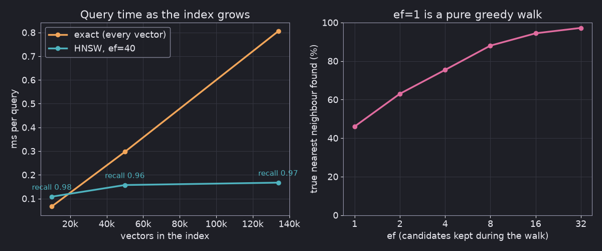
ef is the number of candidates the walk keeps while it searches. With ef=1 it keeps exactly one, so it is a pure greedy walk. That turned out to be a nice demonstration of why greedy algorithms fail:

ef	1	2	4	8	16	32
True nearest neighbour found	46%	63%	75%	88%	94%	97%

A pure greedy walk stops at a vector that is closer than all of its neighbours, but not the closest overall, more than half the time. Keeping a few more candidates fixes most of that, at the cost of more distance computations. Raising ef from 10 to 160 took recall@10 from 0.86 to 0.99 and query time from 0.07 to 0.5 ms.

The index also costs time to build: 19 seconds for 134k vectors here, against zero for exact search. And recall varied by about ±0.02 between our runs, because hnswlib builds the graph with several threads.

So, do you need one?

Your situation	Choice
Up to tens of thousands of vectors	Exact search with NumPy. Simpler, always correct, fast enough
Hundreds of thousands to millions, many queries	An HNSW index (hnswlib, FAISS, or a vector database)
Missing a relevant result is costly	Raise ef and measure recall against exact search on your data
The data changes constantly	Check how your index handles inserts and deletes before you choose

Whatever you pick, measure recall on your data. In an earlier run on random unit vectors (not in the published script), the same settings gave recall@10 of 0.30 at 10,000 vectors and 0.02 at 500,000. A graph walk depends on real data having structure.

Full scripts and raw output: corpus, benchmark, output.

Related: What are embeddings? Semantic search with cosine similarity · Build a local RAG in 50 lines