KFold vs TimeSeriesSplit: how shuffled cross-validation hides time-series leakage

23 Oct 2026 in Machine Learning & Engineering

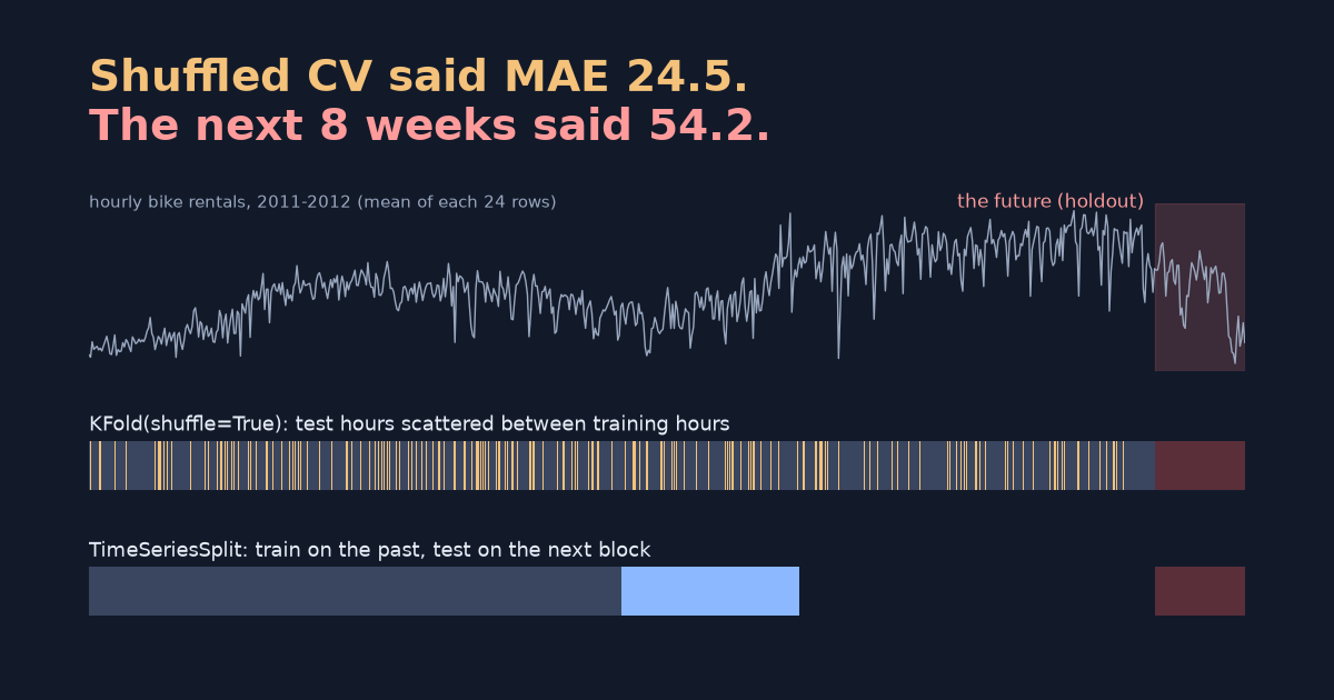
On two years of hourly bike rentals, shuffled KFold estimated MAE 24.5 while the next 8 weeks gave 54.2. When TimeSeriesSplit helps, why lag features change the picture, and the rolling-feature leak no split can catch.

Take one gradient-boosting model, two years of hourly bike rentals, and four cross-validation schemes. Shuffled KFold estimates the mean absolute error (MAE) at 24.5 bikes per hour. Score the same model on the 8 weeks that come after the training data and you get 54.2, more than twice as bad. TimeSeriesSplit estimated 43.4, much closer.

That is the short answer: on time-ordered data, a shuffled split mixes nearby observations into training and test, so the score leans towards “how well can you fill gaps?” instead of “how well can you forecast?”. The experiment also showed two less obvious things. With lag features, shuffled KFold happened to land close to the holdout, and a leaky feature gets straight past TimeSeriesSplit.

Tested on 2026-10-19 with scikit-learn 1.9.1, pandas 3.0.6, NumPy 2.5.4 and Python 3.12.13 on Apple Silicon (macOS). All numbers below come from ts_leakage.py (full output); repeated runs printed identical values.

The setup

The data is the UCI Bike Sharing dataset (Fanaee-T, 2013, CC BY 4.0), loaded from OpenML as Bike_Sharing_Demand version 2: 17,379 hourly rows from 2011 to 2012, in time order. The target is the number of rentals in the hour. A few hours are missing from the data, so one row is usually, but not always, one hour. That matters later.

• “The future”: the last 1,344 rows are held out. That is 8 weeks of rows, covering 1,348 actual hours in November and December 2012. The remaining 15,867 rows are the development set that cross-validation sees (the first 168 rows are dropped because they have no one-week lag).
• Model: HistGradientBoostingRegressor(random_state=0) with default settings.
• Features: calendar and weather columns (season, month, hour, weekday, holiday, temperature, humidity, …), plus t, the row index, as a simple trend feature.

from sklearn.model_selection import KFold, TimeSeriesSplit, cross_validate

SCHEMES = {
    "KFold(5, shuffle=True)": KFold(5, shuffle=True, random_state=0),
    "KFold(5)": KFold(5),
    "TimeSeriesSplit(5)": TimeSeriesSplit(5),
    "TimeSeriesSplit(5, gap=168)": TimeSeriesSplit(5, gap=168),
}
for name, cv in SCHEMES.items():
    r = cross_validate(model(), X_dev, y_dev, cv=cv, scoring="neg_mean_absolute_error")
    print(name, -r["test_score"].mean())

TimeSeriesSplit trains on the first k blocks and tests on block k+1, so the model never trains on anything later than the test block. gap=168 also drops the last 168 rows of each training set, so training ends about a week before the test block starts. Both are described in the scikit-learn documentation (gap was added in version 0.24).

Result 1: without lag features, shuffled KFold is off by a factor of two

Validation	Estimated MAE	Difference from holdout (54.2)
KFold(5, shuffle=True)	24.5	−29.7
KFold(5) (contiguous blocks, no shuffle)	40.2	−14.0
TimeSeriesSplit(5)	43.4	−10.8
TimeSeriesSplit(5, gap=168)	47.4	−6.8
Holdout: the next 8 weeks	54.2	—

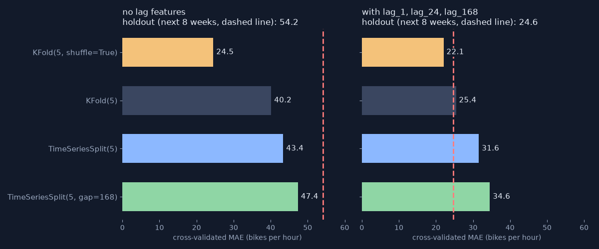
With shuffling, most test hours have training hours from the same day on either side, and demand in neighbouring hours is often similar. Together with t, which tells the model roughly where a row sits in time, that turns the test into interpolation. It is not one lucky fold either: the five shuffled folds scored 24.3 to 25.0.

The time-ordered schemes were still optimistic, by 7 to 11 bikes per hour. One likely reason is that the holdout is a different situation from any test fold: late autumn and winter, with the training data ending just before it. A tree model also cannot extend t past the largest value it saw in training, so the trend stops at the end of the training data. This experiment does not separate those effects; the practical point is that cross-validation of any kind did not replace a final test on the most recent period.

Result 2: with lag features, shuffled KFold happens to land close

Forecasting models usually include recent values of the target. The lag model adds the demand 1, 24 and 168 rows earlier. Because of the missing hours, those are exactly 1, 24 and 168 hours earlier in 99.6%, 90.2% and 68.8% of rows.

Validation	Estimated MAE
KFold(5, shuffle=True)	22.1
KFold(5)	25.4
TimeSeriesSplit(5)	31.6
TimeSeriesSplit(5, gap=168)	34.6
Holdout: the next 8 weeks	24.6

Be precise about what the holdout measures now. The lag columns in the holdout are filled with the real demand as it arrives, and the weather columns are the actual weather. So 24.6 is the error of predicting the next row, one step at a time, with the latest observation and the weather already known. It is not the error of forecasting all 8 weeks in one go, which would be much harder.

Under that setup, shuffled KFold is 2.5 below the holdout and TimeSeriesSplit is 7.0 above it. Two caveats keep this from being a point in favour of shuffling:

• Shuffled KFold still leaks. Lags are computed before splitting, so a training row’s lag_1 can be the target of a test row one hour earlier. The test answer sits inside the training features. Landing close to one holdout does not validate the method.
• TimeSeriesSplit is pessimistic here partly by design. Its first fold trains on only 2,647 rows (about 110 days) and scored 33.7; with the gap, 45.1. Averaging folds trained on much less data than the final model pulls the estimate up.

Result 3: a feature leak that TimeSeriesSplit cannot catch

The split controls which rows the model sees. It does nothing about what is inside each row. A common mistake is a rolling average that includes the current value:

leaky  = y.rolling(3).mean()           # rows t-2, t-1, t   -> contains the answer
honest = y.shift(1).rolling(3).mean()  # rows t-3, t-2, t-1 -> known before row t

Rolling feature (added to the lag model)	TimeSeriesSplit(5) MAE	Holdout MAE
Leaky feature, leaky values	26.5	17.2
Leaky model, served the honest values	—	58.0
Honest feature, retrained	31.5	25.4

The leaky feature looks like an improvement everywhere you test it: cross-validation drops from 31.5 to 26.5 and the holdout from 25.4 to 17.2, because the test rows contain the leaky value too.

In production, the current hour’s demand doesn’t exist yet when you predict it, so the serving code can only compute the honest version. The second row simulates that train/serve mismatch: the model trained on the leaky definition receives the honest values, and the error jumps to 58.0. The fix is not to patch the input but to retrain on the honest feature, which gives 25.4.

This is the same rule as fitting preprocessing on training data only, applied to time: every feature must be computable from information available at prediction time. The non-time version is in Why fit preprocessing on training data only?.

What to use

• Time-ordered data: start with TimeSeriesSplit. It never trains on rows after the test block. Use gap when information arrives late or labels are defined over a future window, for example a target that is “rentals in the next 24 hours”, or sensor data that lands a day late. Lag features built only from past values don’t need a gap by themselves.
• Look at the folds, not only the mean. Early folds train on little data. max_train_size won’t help: it only caps the training size, so the first fold stayed at 2,647 rows even with max_train_size=10000. A smaller test_size will: with test_size=1344 the first fold trains on 9,147 rows. You can also judge mainly by the last folds.
• Keep a final holdout at the end of the timeline and touch it once. Here the cross-validation estimates missed it by 0.8 to 29.7 bikes per hour, in both directions.
• Audit features separately. For every rolling, cumulative or target-encoded column, ask “could I compute this value at the moment of prediction?”. No split strategy answers that question for you.

The same “the split answers a different question” problem shows up with repeated groups instead of time: Before replacing LightGBM with TabPFN-3.5, check your evaluation split shows a random-row split scoring 1.0000 AUC that falls to 0.4748 on unseen groups.

Limits of this test

One dataset, one model and one holdout period, with lag features measured as one-step-ahead prediction. The size of each gap will differ on your data. The direction is the part to expect elsewhere: shuffled splits reward interpolation, and leaky features survive any row split. The tables and charts come from ts_leakage.py and ts_charts.py; the dataset downloads through sklearn.datasets.fetch_openml on the first run.

The experiment code was also reviewed by a second coding agent (OpenAI Codex), which reran it and matched every printed number (how that review was set up).

Related: Train, validation and test sets: what overfitting looks like in numbers · Why you should always build a baseline model first