How many bins should a histogram have?

30 Sep 2026 in HK's DA Note

Too few bins hide the shape of your data, too many turn it into noise. Here is what the common bin rules (sqrt, Sturges, Freedman–Diaconis, auto) actually return, tested with NumPy.

TL;DR — There is no single right number. Start with bins="auto" in NumPy or matplotlib, which picks a width from the data, then compare it with one coarser and one finer setting before you draw conclusions. If the data has a long tail, change the scale (for example, a log axis) instead of fighting with the bin count.

Tested on 2026-09-28 with NumPy 2.5.3, matplotlib 3.11.2, pandas 3.0.6.

Key points

• The default is only 10 bins. Both plt.hist and pandas.Series.hist use bins=10 unless you say otherwise.
• Too few bins hide structure. Too many bins show noise and empty gaps.
• Rules of thumb grow with data size. Most of them scale with the cube root of n; Sturges grows only with log2(n).
• bins="auto" is a good first try. In NumPy it takes the narrower of Sturges and Freedman–Diaconis, with a cap on the bin count.
• Always compare a few settings. A pattern that appears at only one bin count is probably not real.

What happens with too few or too many bins?

The bin count changes what story the chart tells. Here are 1,000 delivery times from two groups: a fast group around 30 minutes and a slow group around 45 minutes.

import numpy as np

rng = np.random.default_rng(7)
# Delivery times (minutes): a fast group and a slow group
x = np.concatenate([rng.normal(30, 4, 600), rng.normal(45, 4, 400)])

for bins in [5, 10, "auto", 200]:
    counts, edges = np.histogram(x, bins=bins)
    print(f"bins={str(bins):<5} -> {len(counts):>3} bins, width {edges[1] - edges[0]:.2f} min, "
          f"empty bins: {(counts == 0).sum()}")

bins=5     ->   5 bins, width 7.66 min, empty bins: 0
bins=10    ->  10 bins, width 3.83 min, empty bins: 0
bins=auto  ->  13 bins, width 2.95 min, empty bins: 0
bins=200   -> 200 bins, width 0.19 min, empty bins: 25

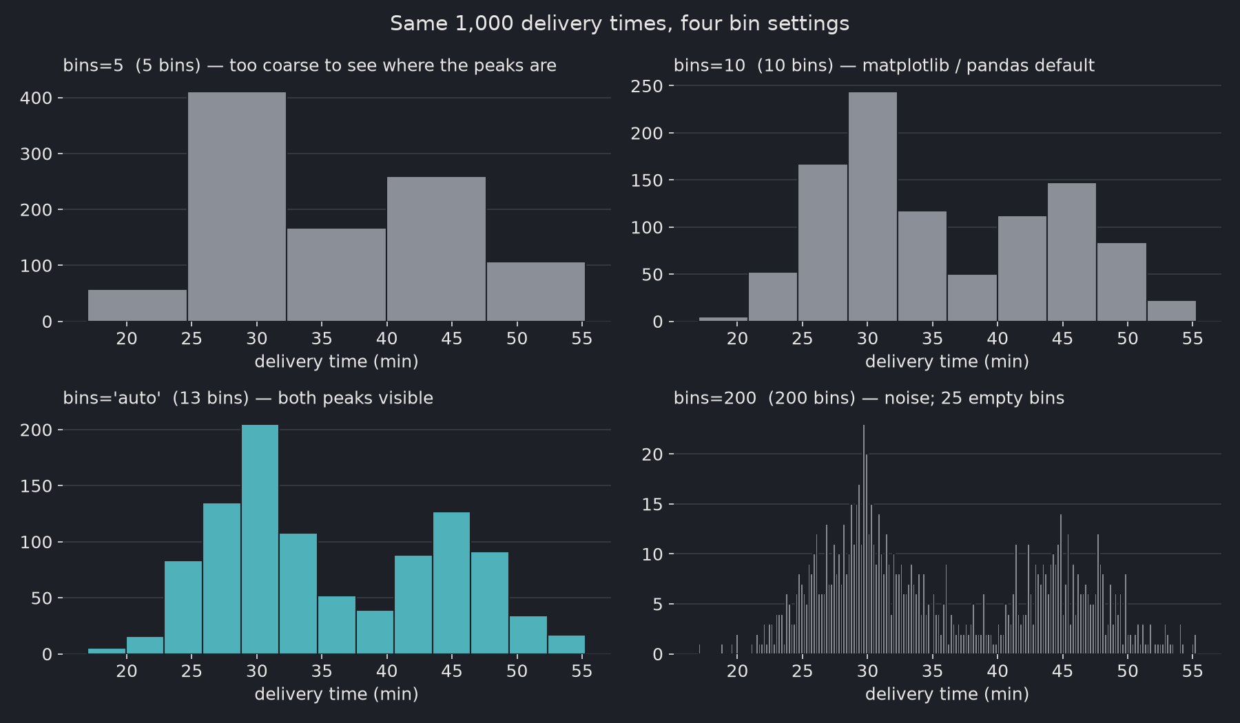
• 5 bins: each bar is 7.7 minutes wide. You can tell there is more than one group, but not where the peaks are.
• 10 bins (the default): both groups show up, but the peak positions are still rough.
• auto (13 bins): clear peaks near 30 and 45 minutes, with a dip between them.
• 200 bins: 25 bins are empty and the bars jump up and down. Most of that is random noise.

What do the common bin rules return?

Each rule turns the data size (and sometimes its spread) into a bin count or a bin width. This code prints the number of bins each NumPy rule picks for normal data of different sizes, and for a long-tailed sample:

import numpy as np

rng = np.random.default_rng(42)
rules = ["sqrt", "sturges", "rice", "scott", "fd", "auto"]

def n_bins(x, rule):
    return len(np.histogram_bin_edges(x, bins=rule)) - 1

print(f"{'data':<18}" + "".join(f"{r:>9}" for r in rules))
for n in [100, 1_000, 100_000]:
    x = rng.normal(50, 10, n)
    print(f"{'normal, n=' + format(n, ','):<18}" + "".join(f"{n_bins(x, r):>9}" for r in rules))
x = rng.lognormal(3, 1, 1_000)
print(f"{'lognormal, n=1,000':<18}" + "".join(f"{n_bins(x, r):>9}" for r in rules))

data                   sqrt  sturges     rice    scott       fd     auto
normal, n=100            10        8       10        8        9        9
normal, n=1,000          32       11       20       20       27       27
normal, n=100,000       317       18       93      125      162      162
lognormal, n=1,000       32       11       20       33       88       64

Rule	Formula (from the NumPy docs)	Behavior in the test above
Square root (sqrt)	bins = √n	Grows fastest: 317 bins at n=100,000
Sturges	bins = log2(n) + 1	Grows slowest: only 18 bins at n=100,000. It assumes normal data
Rice	bins = 2 · n^(1/3)	Ignores the spread of the data
Scott	width = σ · (24√π / n)^(1/3)	Uses the standard deviation, so outliers affect it
Freedman–Diaconis (fd)	width = 2 · IQR / n^(1/3)	Uses the interquartile range, so it resists outliers
auto	Narrower of Sturges and fd, with a cap	Equals fd for normal data from n=1,000 in this test

Two things stand out:

• Sturges falls behind on large data. At n=100,000 it suggests 18 bins while fd suggests 162. Sturges is the default in R’s hist(), so keep this in mind if you compare charts across tools.
• auto has a hidden cap. For the long-tailed sample, fd asks for 88 bins but auto returns 64. In the NumPy 2.5.3 source, auto never makes bins narrower than half the sqrt rule’s width (max(fd_bw, sqrt_bw / 2)). That limits it to about twice the sqrt bin count, here 2 × 32 = 64.

What should you do with long-tailed data?

Change the scale first. When a few values are far larger than the rest, any bin count leaves most bars squeezed on the left:

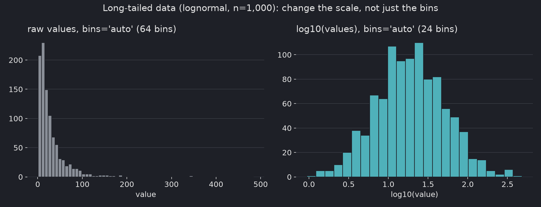
On the raw scale, auto gives 64 bins and almost all of the data sits in the first few bars. After np.log10, auto needs only 24 bins and the shape is easy to read. Income, prices, file sizes, and response times often look like this.

Common mistakes

• Trusting the default. bins=10 is a placeholder, not a choice. Set bins="auto" or a number you have checked.
• Comparing histograms with different bin edges. When you overlay two groups, pass the same bins array to both, for example edges = np.histogram_bin_edges(all_data, bins="auto").
• Reading meaning into one setting. Check that a peak or gap survives a coarser and a finer bin count.
• Using many bins on small data. With 50 normal points and 30 bins, 53–63% of the bars held 0 or 1 values across five random samples.

Sources

• numpy.histogram_bin_edges — bin rules and formulas, NumPy docs, checked 2026-09-28
• numpy/lib/_histograms_impl.py — auto implementation with the bin-count cap, checked 2026-09-28
• matplotlib.pyplot.hist — matplotlib docs

Related: What is a histogram?