Choose a retrieval threshold for cosine similarity

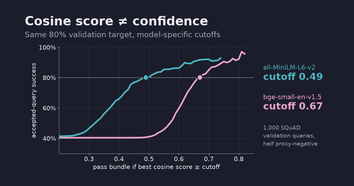
09 Nov 2026 in AI & Developer Tips · Retrieval and RAG

A cosine score of 0.5 does not mean 50% sure. On 2,000 SQuAD questions, half with their gold articles excluded, we pick a “no answer” threshold on validation data, check it on held-out questions, and show why the number does not carry over to another embedding model.

A retrieval step always returns something. Ask a document search about a topic it has never seen and the top result still comes back with a cosine score, say 0.45. A common fix is a cutoff: “if the best score is below X, answer ‘I don’t know’”. The trouble is choosing X. A cosine score is not a probability: 0.45 does not mean 45% sure, and the same score means different things for different models.

With all-MiniLM-L6-v2, the cutoff that gave 80% precision on validation was 0.49. On the test questions it gave 67.6%. Another model needed a cutoff of 0.67 for the same target, and applying MiniLM’s 0.49 to it answered 99% of questions at 41% precision.

SQuAD articles with indexed and excluded sources

Embeddings turn text into vectors, and cosine similarity compares two of them: 1 means the same direction and 0 means orthogonal. Semantic relevance depends on the embedding model. The data is the SQuAD v1.1 dev set (CC BY-SA 4.0): 48 Wikipedia articles, each split into paragraphs, with questions written about each paragraph.

We create proxy-negative questions by leaving whole articles out of the search corpus:

Shuffle the 48 articles (seed 0). Put the paragraphs of 32 of them in the corpus.
Answerable questions come from those 32 articles. Each was written about one paragraph, its right paragraph.
Proxy-negative questions come from the other 16 articles. Their annotated paragraph is absent, so any returned bundle counts as a miss under this exact-source protocol. Other indexed paragraphs might still answer them.
Give validation and test separate articles: validation uses 16 corpus articles plus 8 left-out articles; test uses the other 16 plus 8. Sample 500 answerable and 500 unanswerable questions for each.

The code’s answerable flag means the annotated source is indexed. Printed labels such as no answer in corpus and unanswerable identify the excluded-article proxy. Success means retrieving the annotated paragraph in the three-paragraph bundle; the limits of these labels are discussed below.

To run it yourself, install the packages from requirements.txt, download the dev set, and run the blocks below in order in one Python session. The first run downloads the two models from Hugging Face.

python -m pip install -r requirements.txt
curl -O https://rajpurkar.github.io/SQuAD-explorer/dataset/dev-v1.1.json

import json
import random

import numpy as np
from sentence_transformers import SentenceTransformer

articles = json.load(open("dev-v1.1.json"))["data"]
order = list(range(len(articles)))
random.Random(0).shuffle(order)
groups = {"val": (order[:16], order[32:40]), "test": (order[16:32], order[40:48])}

corpus, questions = [], {}
for split, (in_corpus, left_out) in groups.items():
    answerable, unanswerable = [], []
    for a in in_corpus:
        for p in articles[a]["paragraphs"]:
            corpus.append(p["context"])
            answerable += [(qa["question"], len(corpus) - 1) for qa in p["qas"]]
    for a in left_out:
        unanswerable += [(qa["question"], -1) for p in articles[a]["paragraphs"] for qa in p["qas"]]
    rng = random.Random(1)
    questions[split] = rng.sample(answerable, 500) + rng.sample(unanswerable, 500)
print("corpus paragraphs:", len(corpus))
print({split: len(q) for split, q in questions.items()})

corpus paragraphs: 1439
{'val': 1000, 'test': 1000}

Next, embed the corpus and the questions with all-MiniLM-L6-v2 (Apache-2.0), on CPU. Suppose the answer step reads the top 3 paragraphs. For each question keep the best cosine score and whether the right paragraph is among those 3.

def retrieve(model_name, revision, query_prefix=""):
    model = SentenceTransformer(model_name, revision=revision, device="cpu")
    docs = model.encode(corpus, batch_size=64, normalize_embeddings=True)
    result = {}
    for split, qs in questions.items():
        q = model.encode([query_prefix + text for text, _ in qs], batch_size=64, normalize_embeddings=True)
        sims = q @ docs.T  # cosine similarity, because the vectors are normalized
        top3 = np.argsort(-sims, axis=1)[:, :3]
        gold = np.array([g for _, g in qs])
        result[split] = {"score": sims.max(axis=1), "correct": (top3 == gold[:, None]).any(axis=1),
                         "answerable": gold >= 0}
    return result

mini = retrieve("sentence-transformers/all-MiniLM-L6-v2", "1110a243fdf4706b3f48f1d95db1a4f5529b4d41")
v = mini["val"]
for name, mask in [("right one in top 3", v["correct"]),
                   ("right one missed", v["answerable"] & ~v["correct"]),
                   ("no answer in corpus", ~v["answerable"])]:
    print(f"{name:20s} n={mask.sum():3d}  top-1 score median {np.median(v['score'][mask]):.3f}")

right one in top 3   n=414  top-1 score median 0.605
right one missed     n= 86  top-1 score median 0.561
no answer in corpus  n=500  top-1 score median 0.349

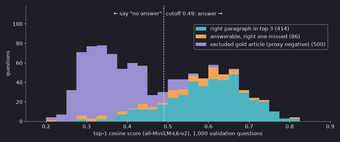
Stacked histogram of best cosine scores for 1,000 validation queries: 500 excluded-article proxy negatives, 414 queries with their annotated paragraph in the top three, and 86 indexed-source misses. A dashed line marks cutoff 0.49; the groups overlap.

The three groups overlap. Excluded-article questions still have a median best score near 0.35. No cutoff cleanly separates these retrieval outcomes. The cover plots validation acceptance curves, omitting cutoffs passing fewer than 20 queries; the curves show source-retrieval success against the 80% target.

Coverage and acceptance precision

For a cutoff t, the gate passes a three-paragraph bundle when its top-1 score is at least t; otherwise it abstains.

Coverage: the share of all queries whose bundle is passed.
Acceptance precision: among passed queries, the share whose bundle contains the annotated paragraph. Excluded-article queries count as misses by construction. The denominator is passed queries, and success requires one annotated paragraph in the bundle. Document precision@3 would count relevant documents among returned documents. Generated-answer accuracy would require evaluating the answer. The code shortens acceptance precision to precision.

A hypothetical perfect retriever and gate could pass all 500 indexed-source queries and reject the 500 proxies: 50% coverage under this labeling protocol. Our actual retriever also misses some indexed sources.

Raising t cannot increase coverage, but precision can go up or down as queries are removed. For this illustration, scan the 0.00–0.99 grid at 0.01 intervals for the lowest cutoff meeting an 80% validation target:

def precision_coverage(t, r):
    if t is None:
        raise ValueError("No validation cutoff met the target; do not evaluate a missing threshold.")
    answered = r["score"] >= t
    precision = r["correct"][answered].mean() if answered.any() else float("nan")
    return precision, answered.mean()

def choose_threshold(r, target=0.80):
    for t in np.round(np.arange(0.0, 1.0, 0.01), 2):
        if precision_coverage(t, r)[0] >= target:
            return t
    return None

for t in [0.3, 0.4, 0.5, 0.6, 0.7]:
    p, c = precision_coverage(t, mini["val"])
    print(f"t={t:.1f}  precision {p:.3f}  coverage {c:.3f}")
t_mini = choose_threshold(mini["val"])
p, c = precision_coverage(t_mini, mini["test"])
print(f"chosen on validation: t={t_mini:.2f}  ->  test precision {p:.3f}, coverage {c:.3f}")

t=0.3  precision 0.465  coverage 0.886
t=0.4  precision 0.660  coverage 0.608
t=0.5  precision 0.802  coverage 0.434
t=0.6  precision 0.863  coverage 0.255
t=0.7  precision 0.921  coverage 0.063
chosen on validation: t=0.49  ->  test precision 0.676, coverage 0.490

On validation the scan lands at 0.49: 80.1% acceptance precision over 442 passed queries (44.2% coverage). On test it passes 490 queries (49.0%) with 67.6% acceptance precision, below the target. Of the 500 excluded-article questions in each split, 84 pass on test versus 29 on validation. The additional accepted proxies account for part of the precision drop on these held-out topics.

If no grid point meets the target, choose_threshold returns None; the evaluation helper raises an explicit error. Use validation evidence to change the retrieval setup or target, and reserve the test set for evaluating the chosen rule.

Seed 0 was fixed before the run, and it turned out to be the worst of ten article splits. Repeating the whole procedure with split seeds 0 to 9, the chosen cutoff ranged from 0.48 to 0.58 and test precision from 67.6% to 88.2% (median 82.3%). Use as much validation data as you can, from the same kind of questions you expect, and recheck after launch.

Source-hit rates within cosine score bands

If best cosine scores were calibrated probabilities of our source-hit event, scores around 0.5 would correspond to that event about half the time. Group the validation questions by their top score and count how often the right paragraph was in the top 3:

r = mini["val"]
for lo in [0.2, 0.3, 0.4, 0.5, 0.6, 0.7]:
    in_bin = (r["score"] >= lo) & (r["score"] < lo + 0.1)
    if in_bin.any():
        print(f"score {lo:.1f}-{lo + 0.1:.1f}: n={in_bin.sum():3d}  right paragraph in top 3: "
              f"{r['correct'][in_bin].mean():.0%}")

score 0.2-0.3: n=114  right paragraph in top 3: 2%
score 0.3-0.4: n=278  right paragraph in top 3: 4%
score 0.4-0.5: n=174  right paragraph in top 3: 30%
score 0.5-0.6: n=179  right paragraph in top 3: 72%
score 0.6-0.7: n=192  right paragraph in top 3: 84%
score 0.7-0.8: n= 59  right paragraph in top 3: 93%

Scores of 0.3 to 0.4 were almost never right (4%), 0.4 to 0.5 were right 30% of the time, and 0.5 to 0.6 were right 72% of the time. If the score were a probability, those bins would sit near 35%, 45% and 55%. Cosine similarity ranks paragraphs for a question. These bins measure the relationship between that score and source hits in the validation set.

bge-small-en-v1.5 needs its own cutoff

Repeat the same steps with bge-small-en-v1.5 (MIT), a model of similar size from a different family, on the same corpus and questions. Its model card asks for an instruction prefix on short queries, so we add it:

bge = retrieve("BAAI/bge-small-en-v1.5", "5c38ec7c405ec4b44b94cc5a9bb96e735b38267a",
               query_prefix="Represent this sentence for searching relevant passages: ")
print(f"bge median top score, no answer in corpus: {np.median(bge['val']['score'][~bge['val']['answerable']]):.3f}")
t_bge = choose_threshold(bge["val"])
for label, t in [(f"MiniLM's cutoff {t_mini:.2f}", t_mini), (f"its own cutoff {t_bge:.2f}", t_bge)]:
    p, c = precision_coverage(t, bge["test"])
    print(f"bge with {label}: test precision {p:.3f}, coverage {c:.3f}")

bge median top score, no answer in corpus: 0.584
bge with MiniLM's cutoff 0.49: test precision 0.410, coverage 0.990
bge with its own cutoff 0.67: test precision 0.740, coverage 0.470

bge’s score distribution is higher in this run: its median best score for excluded-article questions is 0.58, against 0.35 for MiniLM. Reusing 0.49 passes 990 test queries (99.0%) at 41.0% acceptance precision. Its own validation cutoff, 0.67, passes 470 queries (47.0%) at 74.0%. The bge model card likewise recommends choosing a filtering threshold from the score distribution on your own data. These are results for the two configured pipelines, including bge’s query prefix.

The mix of questions matters as well. The evaluation above uses 50% excluded-article proxies. In the test set, keep all 500 indexed-source questions but only 56 proxies (about 10% of the total), and the same MiniLM cutoff gives a different precision:

r = mini["test"]
keep = np.r_[np.arange(500), 500 + np.arange(56)]
mostly_answerable = {key: value[keep] for key, value in r.items()}
p, c = precision_coverage(t_mini, mostly_answerable)
print(f"t={t_mini:.2f} with ~10% unanswerable: precision {p:.3f}, coverage {c:.3f}")

t=0.49 with ~10% unanswerable: precision 0.792, coverage 0.752

Select a cutoff on your validation traffic

Setting, held-out test questions	Cutoff	Precision	Coverage
MiniLM, cutoff chosen on its validation	0.49	67.6%	49.0%
MiniLM, same cutoff, ~10% excluded-article proxies	0.49	79.2%	75.2%
bge, MiniLM’s cutoff reused	0.49	41.0%	99.0%
bge, cutoff chosen on its validation	0.67	74.0%	47.0%
MiniLM, cutoff 0.20 (answers almost everything)	0.20	40.0%	99.7%

Label a validation set from your own traffic, including questions your documents cannot answer. The share of those questions changes precision, so use a realistic mix.
Define success: an acceptance-precision or coverage target, and whether success means a source hit or a correct answer.
Scan cutoffs on validation only, then check the chosen cutoff once on separate test questions.
Choose it again when you change the embedding model, the chunking, or the documents. Use the resulting precision and coverage to decide whether the cutoff fits your system.

The cutoff controls whether the bundle reaches the answer step. If you need a calibrated “how likely is this right” number, fit and evaluate a calibration model with appropriately separated labeled data. A cross-encoder reranker can change the ranking. Validate its scores separately and evaluate calibration if probabilities are needed.

Source labels and split sensitivity

One dataset, two models. SQuAD questions reuse many words from their paragraph, and MiniLM’s training data includes the SQuAD 2.0 training set, per its model card. Questions from real users may be harder; we did not test that.
“Right” means the paragraph the question was written for is in the top 3. Another paragraph may also contain the answer and is counted as wrong, so precision here leans low. Left-out articles could also share facts with the corpus.
The gate looks only at the best score. It does not check whether the answer step actually uses the paragraph.
The setup was revised once after a first look at this data. Counting only the single best paragraph, no cutoff reached 80% precision on validation, so we switched to the top-3 rule and set the 80% target. bge was chosen as the second model because its scores sit on a visibly different scale; the size of the gap depends on the models compared.
500 + 500 questions per split. Across all ten article splits (seeds 0–9), cutoffs ranged from 0.48 to 0.58 and test acceptance precision from 67.6% to 88.2%; seed 0 was the lowest. These overlapping split experiments share articles and therefore measure sensitivity to the split; they provide neither ten independent samples nor a confidence interval.

Tested on 2026-11-01 with Python 3.12.13, sentence-transformers 6.2.0, transformers 5.22.1, PyTorch 2.15.0 (CPU) and NumPy 2.5.4 on macOS, Apple M5. The full script, including both models, the chart and the ten-split check, took 106 to 123 seconds on CPU in three runs with the models already downloaded, and peaked under 2.1 GiB resident memory. Model revisions are pinned in the code. cosine_threshold.py also writes the scores and chart data; its recorded output is in reference_output.txt.

For other ways to improve what retrieval returns, see hybrid search with BM25.