How to check if data is normally distributed in Python
Q-Q plots, Shapiro-Wilk and D’Agostino tests in SciPy, and why the same near-normal data passes at n=300 but fails at n=3,000. Tested with SciPy 1.18.
TL;DR — Look first, test second. A Q-Q plot shows how your data departs from normal; a test such as scipy.stats.shapiro only says whether it can detect a departure, and that depends heavily on sample size. In our test, the same slightly heavy-tailed distribution passed at 300 points and failed badly at 3,000.
Tested on 2026-09-28 with SciPy 1.18.1, NumPy 2.5.3, Python 3.12.
Key points
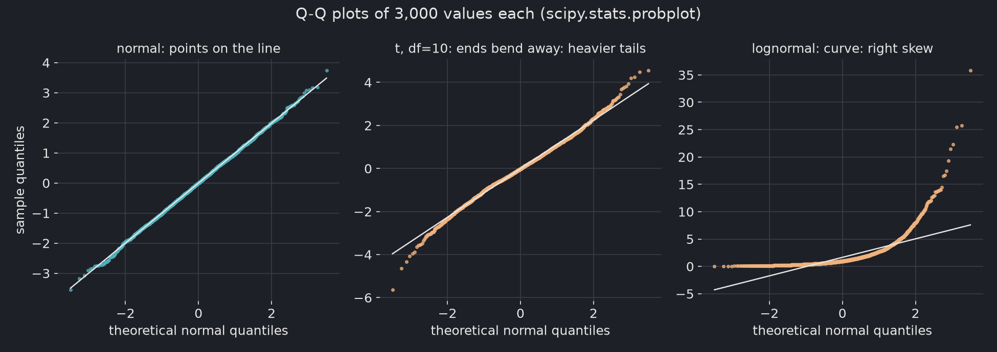
- Q-Q plot: points on the straight line mean normal; bent ends mean heavy or light tails; a curve means skew.
- Shapiro-Wilk (
stats.shapiro) and D’Agostino-Pearson (stats.normaltest) test the null hypothesis “the data is normal”. A small p-value (say < 0.05) means “not normal”. - Large samples reject tiny, harmless deviations. Small samples miss real ones.
- Skewness and kurtosis put a number on the shape: both are about 0 for normal data.
- SciPy warns that Shapiro-Wilk p-values may not be accurate above 5,000 points.
How do you make a Q-Q plot?
A Q-Q (quantile-quantile) plot puts your sorted data against the values a normal distribution would give. scipy.stats.probplot does the math:
import numpy as np
from scipy import stats

rng = np.random.default_rng(1)
samples = {"normal": rng.normal(size=3_000),
           "t, df=10": rng.standard_t(10, size=3_000),
           "lognormal": rng.lognormal(size=3_000)}

(osm, osr), (slope, intercept, r) = stats.probplot(samples["t, df=10"], dist="norm")
# plot osm (x) against osr (y), and the line slope * osm + intercept
| Q-Q pattern | Meaning |
|---|---|
| Points on the line | Close to normal |
| Both ends bend away from the line (S shape) | Heavier tails than normal: more extreme values |
| One-sided curve | Skewed: a long tail on one side |
| Steps or flat runs | Rounded or repeated values |
What do the normality tests say?
Both tests take an array and return a p-value. Here they run on three distributions at four sample sizes:
import warnings
import numpy as np
from scipy import stats

rng = np.random.default_rng(0)
print(f"{'data':<24}{'n':>7}{'Shapiro p':>11}{'normaltest p':>14}")
for label, draw in [("normal", lambda n: rng.normal(size=n)),
                    ("t, df=10 (near-normal)", lambda n: rng.standard_t(10, size=n)),
                    ("lognormal (skewed)", lambda n: rng.lognormal(size=n))]:
    for n in [30, 300, 3_000, 30_000]:
        x = draw(n)
        with warnings.catch_warnings():
            warnings.simplefilter("ignore")      # hides the N > 5000 warning; see below
            p_sw = stats.shapiro(x).pvalue
        p_da = stats.normaltest(x).pvalue
        print(f"{label:<24}{n:>7}{p_sw:>11.3g}{p_da:>14.3g}")
data                          n  Shapiro p  normaltest p
normal                       30      0.688         0.555
normal                      300       0.44         0.305
normal                     3000      0.442         0.383
normal                    30000      0.617         0.396
t, df=10 (near-normal)       30       0.35         0.492
t, df=10 (near-normal)      300      0.911         0.465
t, df=10 (near-normal)     3000   7.67e-07      7.86e-09
t, df=10 (near-normal)    30000   1.29e-29     3.45e-103
lognormal (skewed)           30   0.000237      2.56e-06
lognormal (skewed)          300   7.24e-24      3.67e-62
lognormal (skewed)         3000    2.2e-63             0
lognormal (skewed)        30000  9.37e-122             0
- Normal data passes at every size, as it should.
- Lognormal data fails at every size, even 30. The skew is too strong to miss.
- The t-distribution passes at 30 and 300, then fails at 3,000 and 30,000. The distribution didn’t change. The test just gained enough data to see its slightly heavier tails.
The Shapiro-Wilk results for 30,000 points come with a SciPy warning: For N > 5000, computed p-value may not be accurate. For large samples, rely on normaltest and the Q-Q plot.
How far from normal is the data?
A p-value can’t tell you that. Skewness and excess kurtosis can:
# continues from the Q-Q plot code (samples, stats)
for name, x in samples.items():
    print(f"{name:<10} skewness {stats.skew(x):6.2f}   excess kurtosis {stats.kurtosis(x):6.2f}")
normal     skewness  -0.00   excess kurtosis   0.02
t, df=10   skewness  -0.03   excess kurtosis   0.84
lognormal  skewness   4.86   excess kurtosis  40.60
The t-distribution is symmetric (skewness about 0) with somewhat heavier tails (kurtosis 0.84). The lognormal is in a different league. Whether 0.84 matters depends on what you do next, for example how sensitive your model or test is to extreme values. A p-value of 1e-29 doesn’t answer that.
Which check should you use?
| Situation | Use |
|---|---|
| Any sample size, first look | Q-Q plot plus a histogram |
| Small sample (under ~50) | Q-Q plot and Shapiro-Wilk, knowing the test has little power |
| Large sample (thousands+) | Q-Q plot, skewness and kurtosis; treat test p-values with caution |
| Report or checklist requires a test | stats.normaltest (returns NaN below 8 values) or stats.shapiro (up to ~5,000) |
Sources
scipy.stats.shapiro,scipy.stats.normaltest,scipy.stats.probplot— SciPy docs, checked 2026-09-28
Related: Histogram vs KDE: how do you choose the bandwidth? · How many bins should a histogram have?