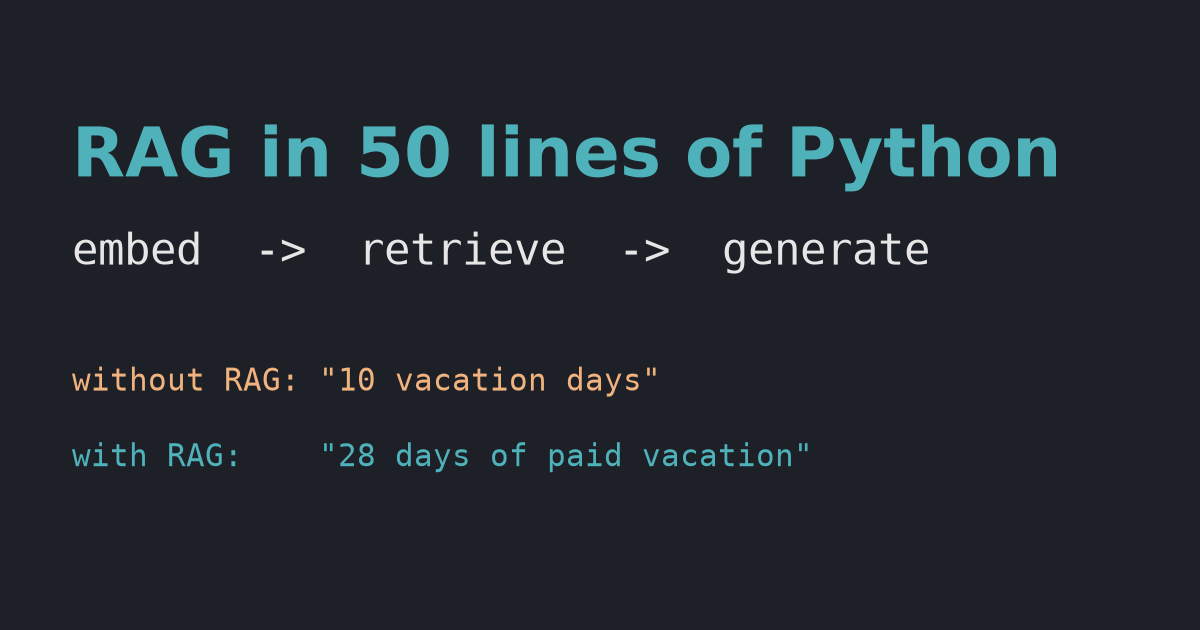
Retrieval-augmented generation in 49 lines: embed documents, retrieve the closest ones, and put them in the prompt. Without RAG, a local model invented a vacation policy; with RAG it answered correctly, and one rule stopped it guessing.
TL;DR — RAG (retrieval-augmented generation) means: find the pieces of your documents that match the question, paste them into the prompt, and ask the model to answer from them. Asked about a fictional company without RAG, a small local model invented answers (“10 vacation days”); with RAG, it answered correctly (“28 days”). When the answer wasn’t in the documents, it still invented one until we told it to say “I don’t know”.
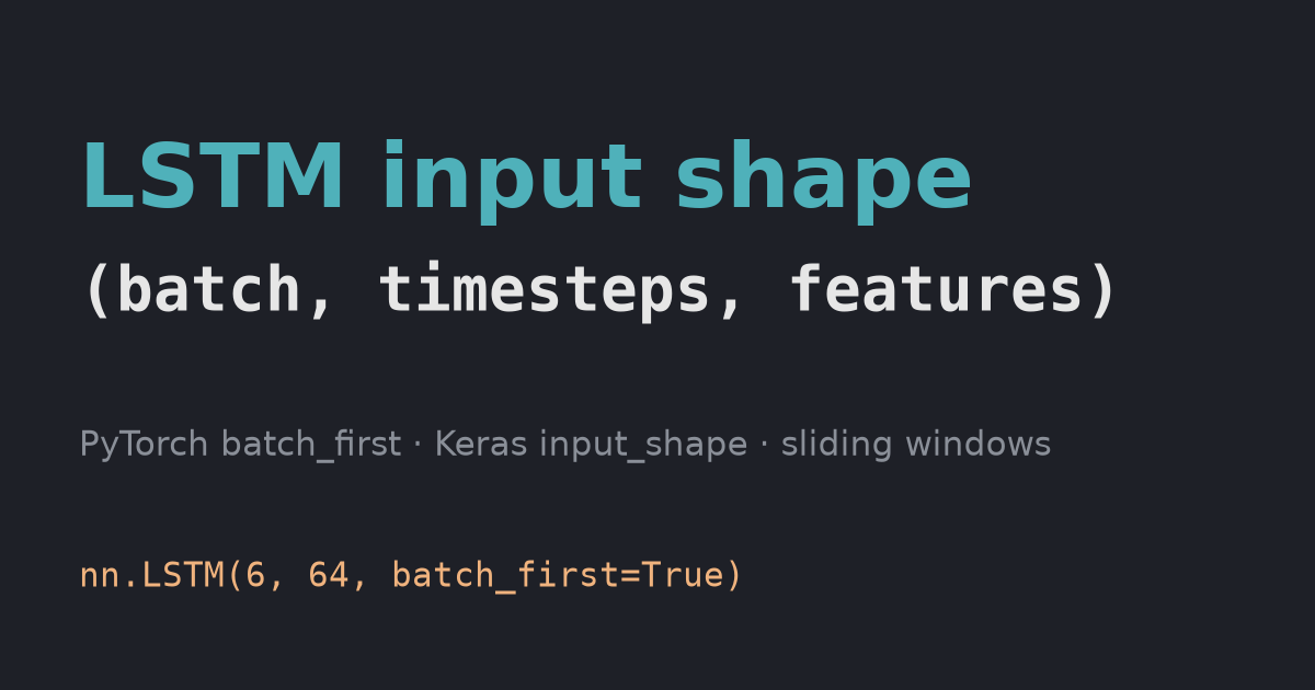
What each of the three LSTM input dimensions means, how to build them from a time series with sliding windows, and the PyTorch batch_first default that silently mixes your samples. Tested with PyTorch 2.14 and Keras 3.15.
TL;DR — An LSTM expects a 3D input: (batch, timesteps, features). Batch is how many sequences you feed at once, timesteps is how many steps each sequence has, and features is how many values you have per step. In PyTorch, pass batch_first=True. Without it, nn.LSTM reads the first dimension as time, and a wrong order runs without any error.
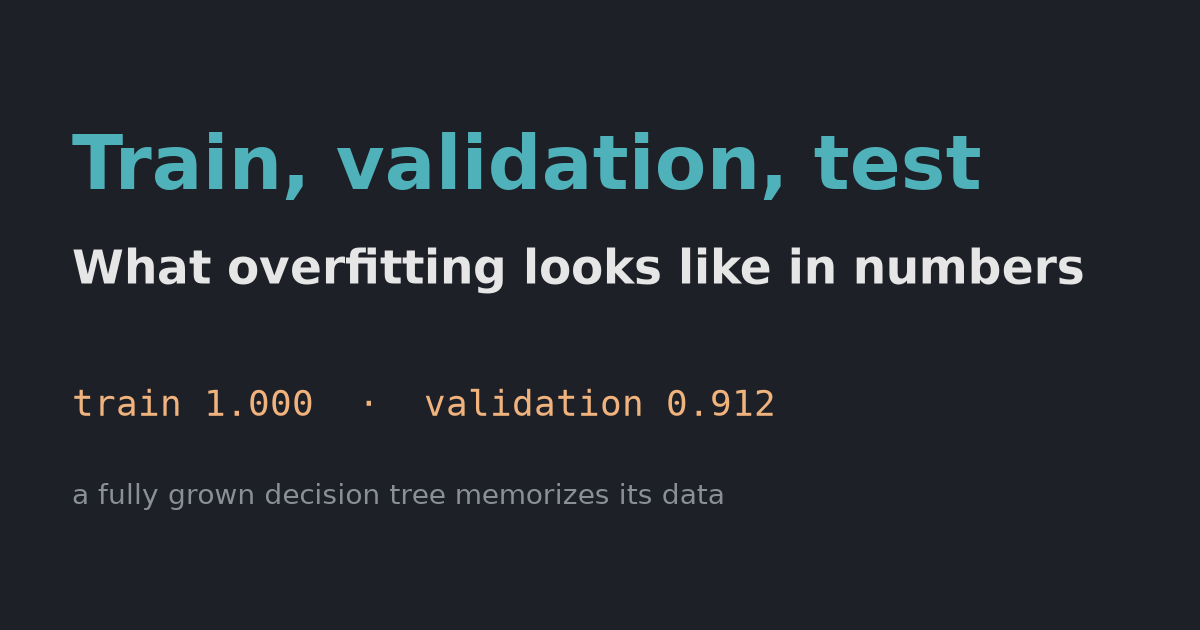
Why you need three data splits, measured on a real dataset: a fully grown decision tree scored 1.000 on training data and 0.912 on validation, and picking the best model on one small validation split overstated the test score.
TL;DR — Train on the training set, choose settings with the validation set (or cross-validation), and use the test set once, at the very end. Overfitting is when a model learns its training data too well to generalize: in our test, a decision tree reached 1.000 training accuracy while validation accuracy fell to 0.912.
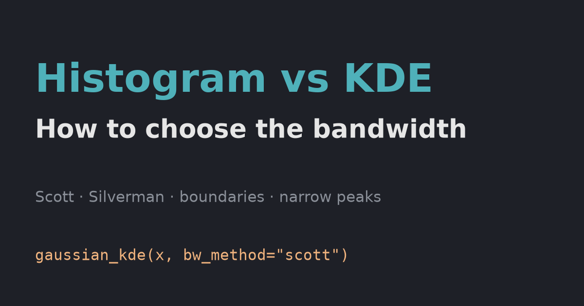
A KDE is a smooth histogram, and its bandwidth works like the bin width. Tested with SciPy: what Scott’s rule gets right, how a KDE leaks below zero, and when a histogram shows more.
TL;DR — Start with the default (Scott’s rule, bw_method="scott" in SciPy), then check it against a histogram. A bandwidth that is too small invents peaks; one that is too large merges real ones. Be careful with data that has a hard limit such as zero, and with narrow spikes: a default KDE handles both poorly.
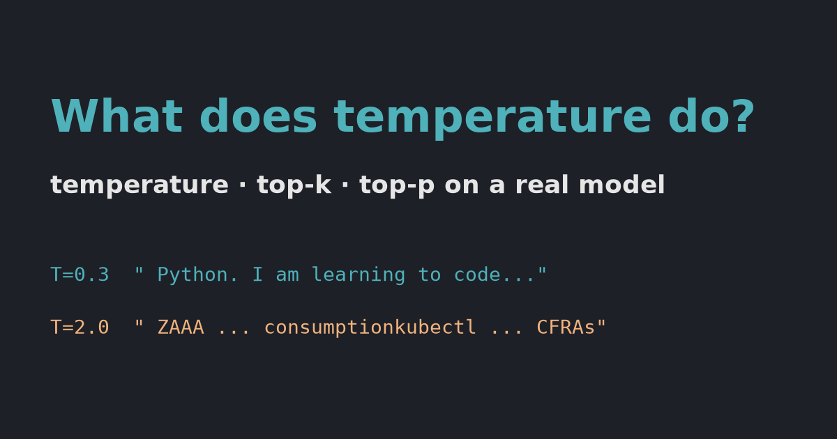
Temperature reshapes the next-token probabilities; top-k and top-p cut off unlikely tokens. Tested on a small open model: at temperature 2.0 the output turned into noise, and top-k fixed it while top-p did not.
TL;DR — An LLM picks each next token by sampling from a probability distribution. Temperature sharpens (below 1) or flattens (above 1) that distribution. Top-k keeps only the k most likely tokens; top-p keeps the smallest set whose probabilities add up to p. Low temperature gives safe, repetitive text; high temperature gives variety, and past a point, noise.
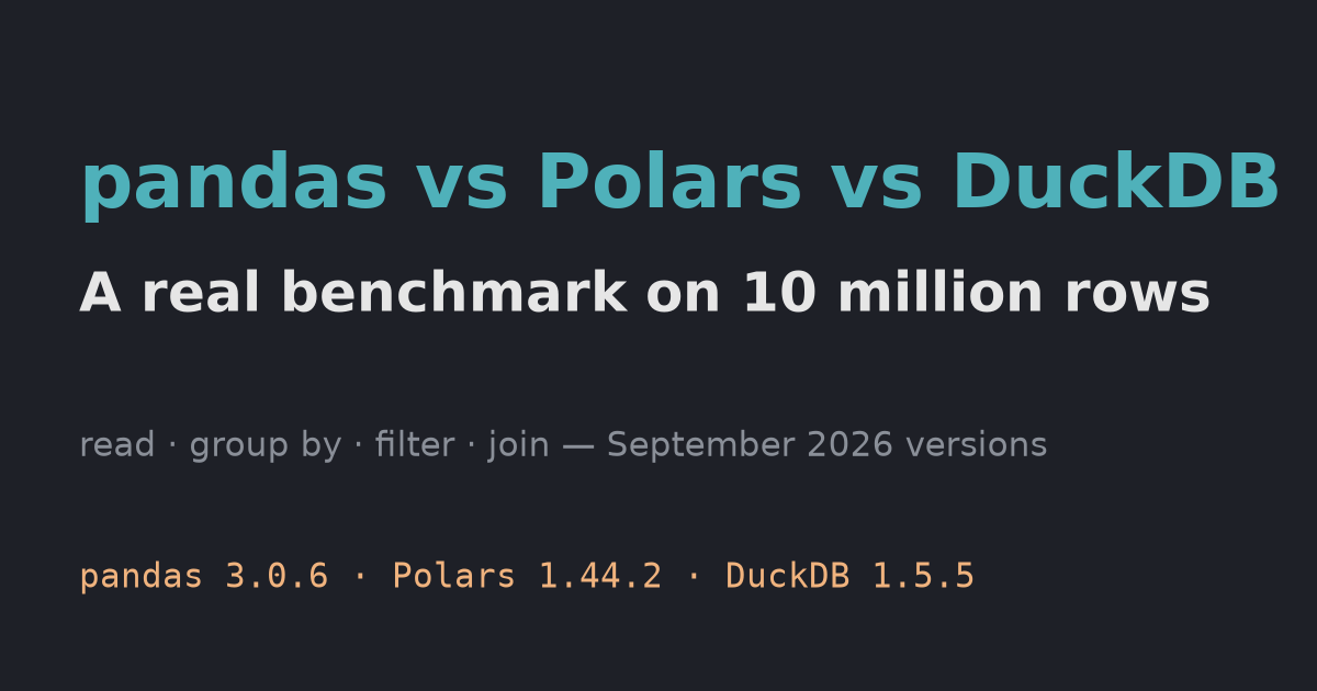
pandas 3.0.6, Polars 1.44.2 and DuckDB 1.5.5 on the same 10M-row dataset: read, group by, filter and join, plus a single-thread run that shows how much of the gap is just parallelism.
TL;DR — On 10 million rows, Polars and DuckDB were 2× to 60× faster than pandas at group by, filter and join. Much of that gap comes from using all CPU cores: limited to one thread, Polars was only about 1.4× to 1.6× faster than pandas. DuckDB’s join stood out, staying fast even on a single thread.
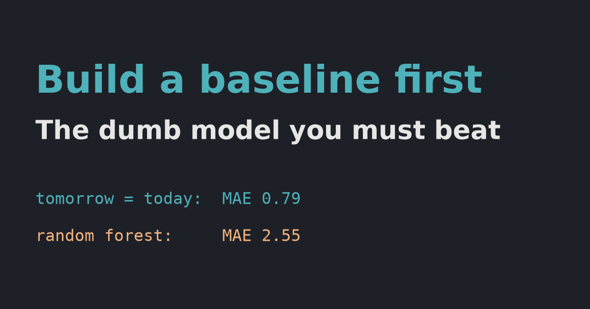
Before training a real model, measure the simplest possible one. On a price-like series, “tomorrow = today” beat a random forest by more than 3×. Tested with scikit-learn, with the reason the forest failed.
TL;DR — A baseline is the simplest prediction you could make without machine learning, such as “tomorrow equals today” or “always predict the average”. Measure it first. If your model can’t beat it clearly, the model isn’t learning anything useful. In our test, the naive baseline scored an error of 0.79; a random forest scored 2.55.
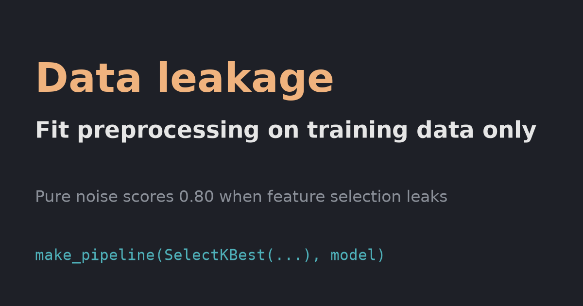
Fitting a scaler or a feature selector on all your data before cross-validation leaks test information. On pure noise, leaky feature selection scored 0.80 instead of 0.50. Tested with scikit-learn 1.9.1.
TL;DR — Any step that learns from data (a scaler, an imputer, a feature selector) must be fitted on the training data only. Otherwise your test score includes information the model won’t have in production. The simplest fix is to put every step in a scikit-learn Pipeline and cross-validate the whole pipeline.
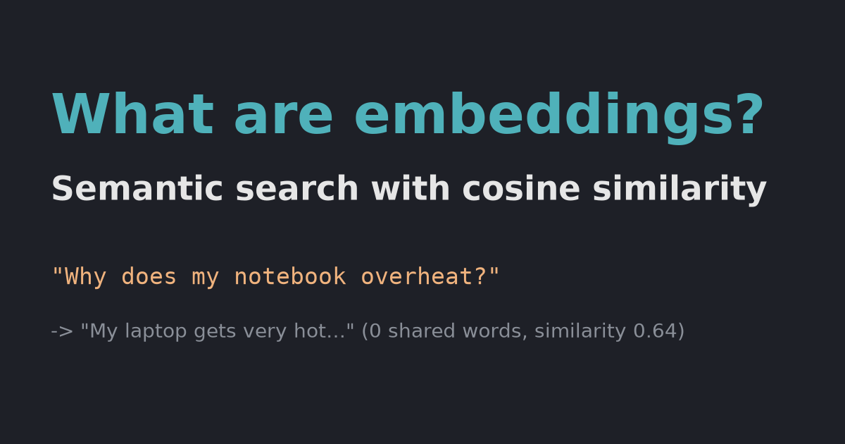
An embedding turns text into a vector so that similar meanings land close together. A 30-line example with a free local model finds “My laptop gets very hot” for “Why does my notebook overheat?”, with no shared words.
TL;DR — An embedding model turns a piece of text into a list of numbers (a vector) so that texts with similar meaning get similar vectors. Comparing vectors with cosine similarity lets you search by meaning instead of by matching words. In our test, keyword search ranked a sourdough sentence first for a laptop question; embedding search found the right answers.
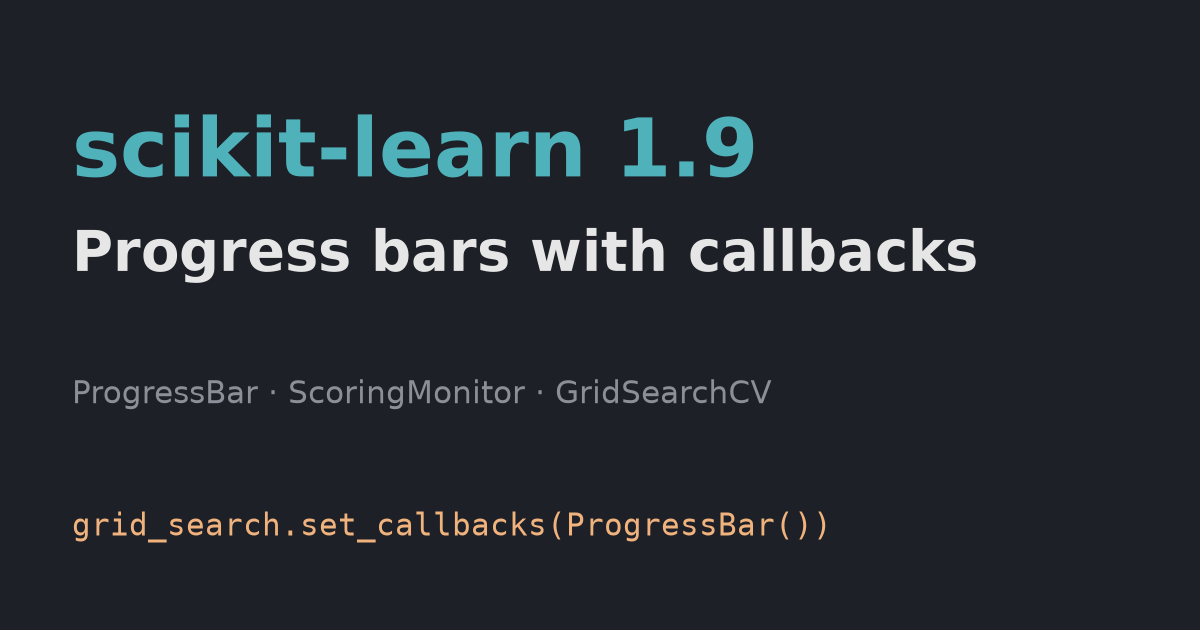
scikit-learn 1.9 added experimental callbacks: ProgressBar for GridSearchCV and Pipeline, and ScoringMonitor for per-iteration training scores. Tested on 1.9.1, including the missing rich dependency.
TL;DR — Since scikit-learn 1.9, you can call grid_search.set_callbacks(ProgressBar()) before fit() to get live progress bars for every candidate and fold. Install rich first (pip install rich), or you get an ImportError. The feature is experimental and works only on a handful of estimators so far.