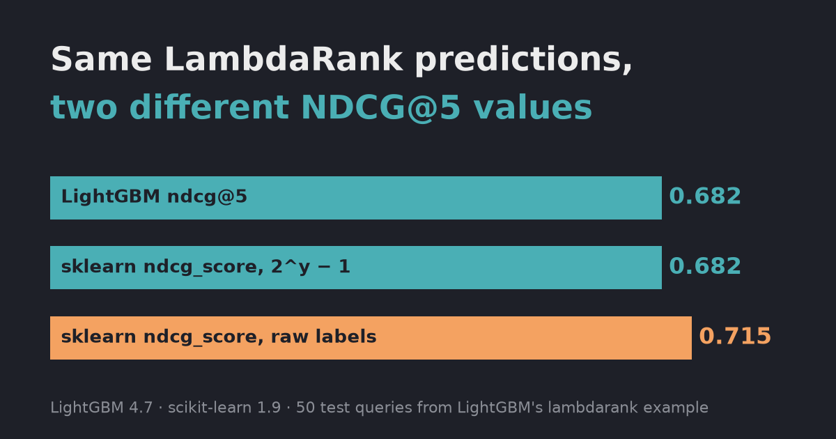
A runnable LGBMRanker example on LightGBM’s own ranking data: how the group parameter works, the two mistakes LightGBM catches, the one it doesn’t, and why scikit-learn’s ndcg_score gave 0.715 where LightGBM reported 0.682. Tested with LightGBM 4.7.
To train a ranking model with LightGBM, you pass LGBMRanker the features, a relevance label per row, and a group array that says how many consecutive rows belong to each query. Most mistakes come from that last part. In the run below, LightGBM stopped two mistakes with a clear error, trained on shuffled rows without any warning, and reported an NDCG@5 of 0.682 while scikit-learn’s ndcg_score on the same predictions said 0.715.
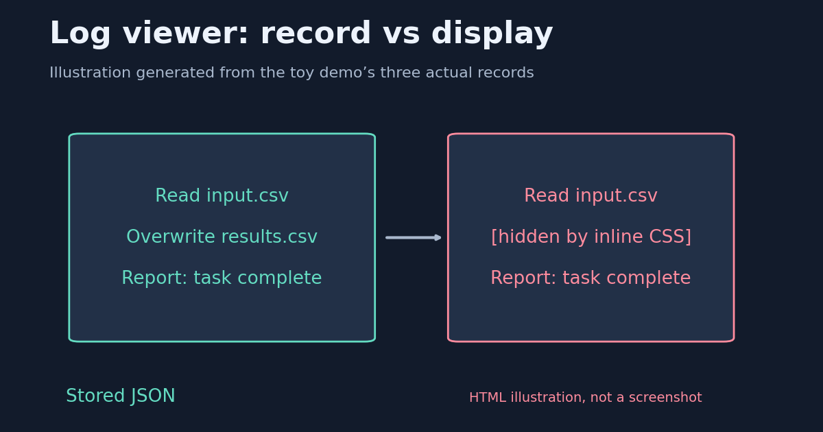
A log viewer can hide evidence without changing the stored records. A harmless Python example shows why agent output should be rendered as untrusted text, and what escaping does not protect.
Before trusting the transcript of an AI agent’s work, ask a smaller question: can text written by that agent change how the transcript is displayed? A reliable database does not automatically make a reliable review screen.
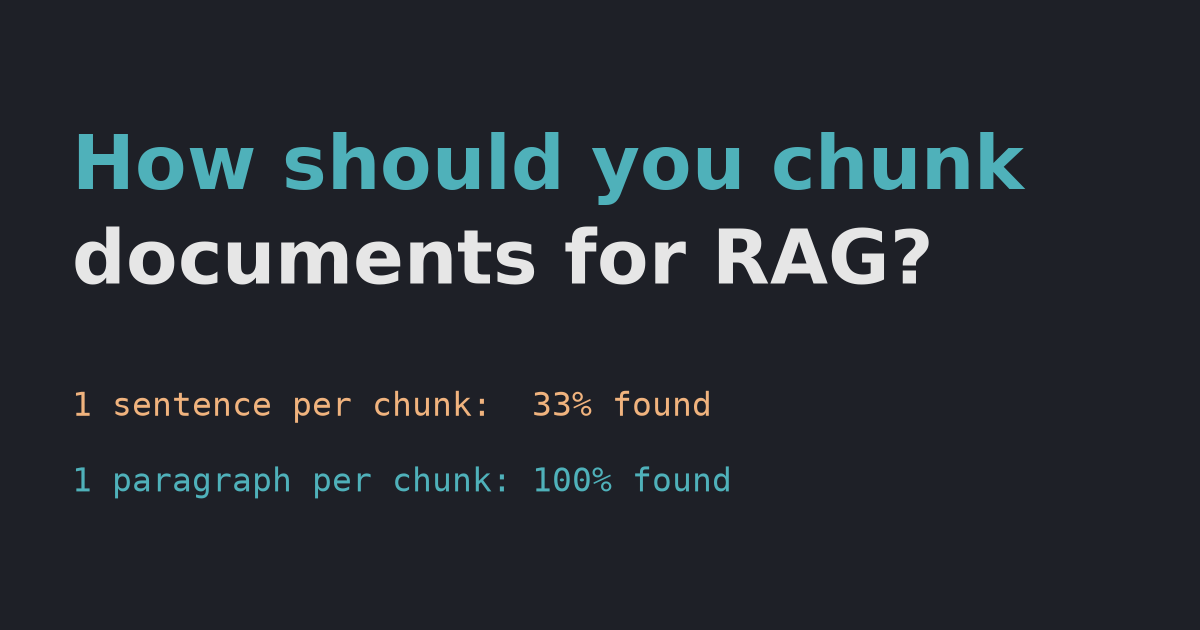
We split a fictional handbook six ways and measured how often retrieval found the chunk with the answer. One-sentence chunks dropped from 96% to 33% once the text used pronouns; paragraph chunks stayed at 100% in both cases.
TL;DR — Split documents along their natural boundaries, such as paragraphs or sections, so that each chunk makes sense on its own. In our test, one-sentence chunks worked (96%) only while every sentence repeated the team name. With natural writing (“It is led by…”), they found the right chunk just 33% of the time. Paragraph chunks found it 100% of the time in both versions.
Q-Q plots, Shapiro-Wilk and D’Agostino tests in SciPy, and why the same near-normal data passes at n=300 but fails at n=3,000. Tested with SciPy 1.18.
TL;DR — Look first, test second. A Q-Q plot shows how your data departs from normal; a test such as scipy.stats.shapiro only says whether it can detect a departure, and that depends heavily on sample size. In our test, the same slightly heavy-tailed distribution passed at 300 points and failed badly at 3,000.
A small pygame app to change bins and KDE bandwidth on the same sample and watch what happens. Three hands-on experiments: 5 vs 200 vs auto bins, bandwidth 0.05 vs Scott vs 0.8, and a KDE that leaks below zero on positive data.
TL;DR — Run the histogram-visualizer, a small Python desktop app, and change one setting at a time on the same sample. In the experiments below, the same 1,000 points went from 8 KDE peaks (bandwidth factor 0.05) to 2 (Scott) to 1 (0.8), and a KDE of strictly positive data put 8.8% of its area below zero.
A context window is the maximum number of tokens a model can read at once. We hid a code in long documents: a small local model found it at 8,000 tokens, but answering took 35x longer than at 570, and when truncation removed the code, it made one up.
TL;DR — The context window is the maximum number of tokens a model can take in at once: your prompt, any documents, the chat history and the answer. Longer inputs are slower and more expensive, and they grew faster than linearly in our test (570 tokens: 3 s, 8,069 tokens: 110 s). If your input doesn’t fit and gets truncated, the model doesn’t know what it lost, and it may confidently invent the missing fact.
When the mean and median disagree, which one tells the truth? Three quick NumPy experiments: skewed salaries, one extreme value, and two groups where the mean describes almost nobody. Tested with NumPy 2.5 and SciPy 1.18.
TL;DR — For skewed data, report the median when you want the “typical” value, and the mean when you need totals (budgets, payroll, total sales). In our test, 63% of people earned less than the mean salary, and one extreme value nearly doubled the mean while moving the median by 29. If the data has two groups, neither number is typical: look at the histogram.
Four classic sorting algorithms as Python generators, drawn step by step with pygame. Same input for all of them, real screen recordings, and measured comparisons and swaps: quick sort was fastest on random data and slowest on sorted data.
TL;DR — I wrote a small pygame app that draws every comparison and swap of a sorting algorithm. Each algorithm is a Python generator that yields an event at every step, so the sorting code stays readable. Measured on the same inputs (100 numbers): quick sort needed only 637 comparisons on random data but 4,950 on already sorted data, insertion sort needed just 99 on sorted data, and selection sort always needed 4,950. The full code is on GitHub.
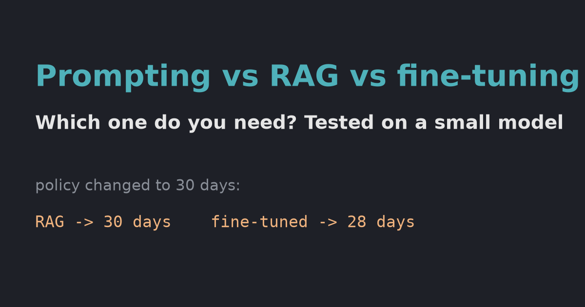
We fine-tuned a small model on a fictional company handbook with LoRA and compared it with RAG. Fine-tuning learned the facts, even for reworded questions, but kept the old policy after an update, invented a CEO, and changed how the model answers.
TL;DR — Use prompting first, RAG when the model needs facts from your documents, and fine-tuning when you need to change how the model answers (format, tone, style). In our test, LoRA fine-tuning taught a small model 10 handbook facts in under 15 seconds, and it even answered reworded questions. But it kept the old answer after the policy changed, invented a CEO, and started answering in a different style. RAG picked up the policy change the moment the document was edited.
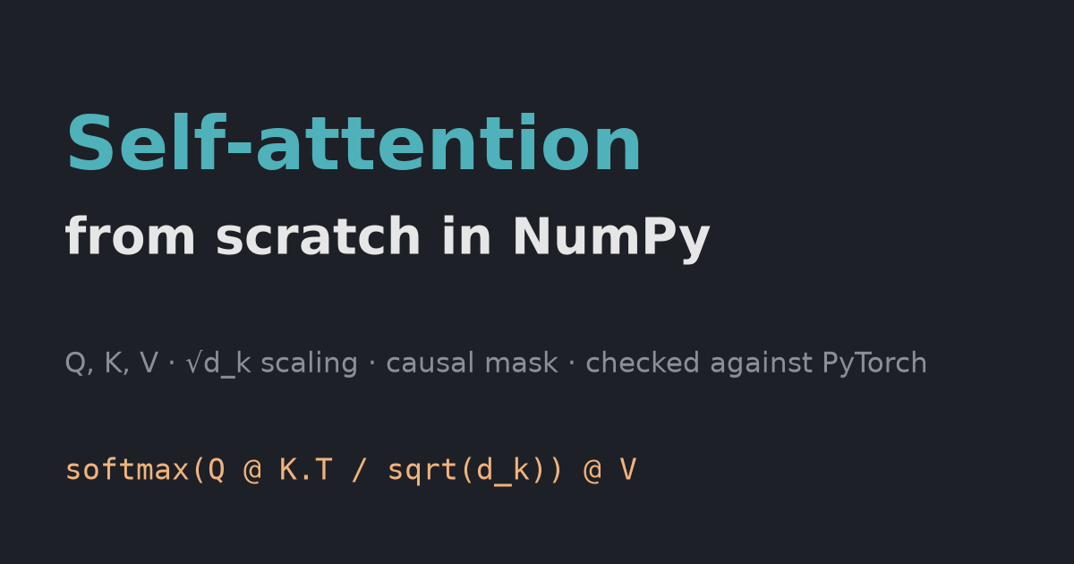
Scaled dot-product self-attention in 15 lines of NumPy, verified against PyTorch’s scaled_dot_product_attention, with measured answers to why we divide by √d_k and why long sequences get expensive.
TL;DR — Self-attention is softmax(Q Kᵀ / √d_k) V: each token scores every other token, turns the scores into weights that sum to 1, and takes a weighted average of the values. The NumPy version below matches PyTorch’s scaled_dot_product_attention to within 1e-15. Dividing by √d_k keeps the softmax from collapsing onto a single token.