Building a scikit-learn Preprocessing Pipeline
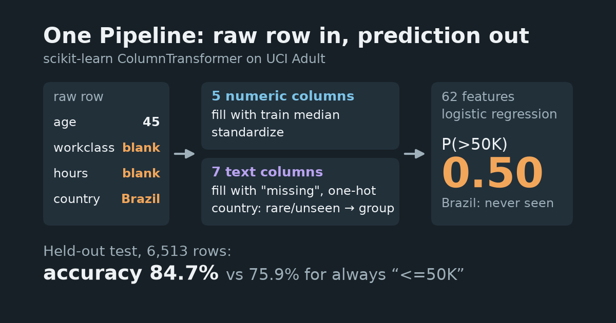
Build one scikit-learn Pipeline that imputes missing values, scales numbers and one-hot encodes categories, then predicts on raw new rows, including a country the model never saw. Real UCI Adult data, a held-out test set, a majority-class baseline and complete runnable code.
In this tutorial you will build one object that takes a raw table row and returns a prediction. The row can contain text categories, blank fields and even a category the model never saw in training. Inside the object, a ColumnTransformer fills the gaps, scales the numeric columns and one-hot encodes the text columns. A logistic regression then makes the prediction. You need basic pandas and a rough idea of a train/test split. No GPU or API key is needed.
The result first: on 6,513 held-out rows, the pipeline predicted the income class correctly for 84.7% of them. Always guessing the most common class scored 75.9%. Then we send it a person from Brazil, a country that is not in the training data. The pipeline still returns an answer instead of crashing. It does not know anything about Brazil, though, and the last steps show what that answer is based on.
1. Set up the environment
Tested on 2026-11-01 with Python 3.12.13, scikit-learn 1.9.1, pandas 3.1.0, NumPy 2.5.4, Matplotlib 3.11.2 and joblib 1.6.0 on macOS, Apple M5 (CPU). A cached-data run of the full script took 2.01 seconds wall time and 243,417,088 bytes (about 232 MiB) peak resident memory. Package installation and the first data download are not included. These are measurements on this machine, not runtime guarantees.
Download pipeline_tutorial.py and requirements.txt into an empty folder, then run:
python3.12 -m venv .venv
source .venv/bin/activate
python -m pip install -r requirements.txt
python pipeline_tutorial.py
The script downloads the data on its first run and writes its outputs under results/. The steps below are the same code split into blocks. Run them in order in one Python session, or paste them into one file. The full script also prints the package versions and draws the chart.
import io
import urllib.request
import zipfile
from pathlib import Path

import joblib
import numpy as np
import pandas as pd
from sklearn.compose import ColumnTransformer
from sklearn.dummy import DummyClassifier
from sklearn.impute import SimpleImputer
from sklearn.linear_model import LogisticRegression
from sklearn.metrics import accuracy_score, roc_auc_score
from sklearn.model_selection import train_test_split
from sklearn.pipeline import Pipeline
from sklearn.preprocessing import OneHotEncoder, StandardScaler

OUT = Path("results")
OUT.mkdir(exist_ok=True)
SEED = 0
2. Download and load the data
We use the UCI Adult dataset by Barry Becker and Ronny Kohavi (1996), DOI 10.24432/C5XW20, licensed CC BY 4.0. It holds records from the 1994 US Census. Each row is one person, and the task is to predict whether that person earned more than $50K a year. It is a teaching dataset with a known history, not a guide to how incomes work today.
The archive has no header row, so we pass the column names from its adult.names file. Missing values are written as ?, so we tell pandas to read ? as missing.
URL = "https://archive.ics.uci.edu/static/public/2/adult.zip"
COLUMNS = ["age", "workclass", "fnlwgt", "education", "education-num", "marital-status",
           "occupation", "relationship", "race", "sex", "capital-gain", "capital-loss",
           "hours-per-week", "native-country", "income"]
archive = OUT / "adult.zip"
if not archive.exists():
    request = urllib.request.Request(URL, headers={"User-Agent": "Pipeline-Tutorial/1.0"})
    with urllib.request.urlopen(request, timeout=60) as response:
        archive.write_bytes(response.read())
with zipfile.ZipFile(io.BytesIO(archive.read_bytes())) as zipped:
    df = pd.read_csv(zipped.open("adult.data"), names=COLUMNS,
                     skipinitialspace=True, na_values="?")
df = df.dropna(how="all")  # guard against a trailing blank line
print(df.shape)
print(df["income"].value_counts().to_string())
(32561, 15)
income
<=50K    24720
>50K      7841
The archive also contains adult.test. We do not use it here: one file and our own split keep the tutorial short.
3. Look at the problems before fixing them
Check three things: which columns have gaps, whether rows repeat, and how often each category appears.
missing = df.isna().sum()
print(missing[missing > 0].to_string())
print("Duplicate rows:", df.duplicated().sum())
countries = df["native-country"].value_counts()
print("Countries:", len(countries), "| with fewer than 50 rows:", (countries < 50).sum())
print(countries.iloc[[0, 1, -3, -2, -1]].to_string())
workclass         1836
occupation        1843
native-country     583
Duplicate rows: 24
Countries: 41 | with fewer than 50 rows: 20
native-country
United-States         29170
Mexico                  643
Hungary                  13
Scotland                 12
Holand-Netherlands        1
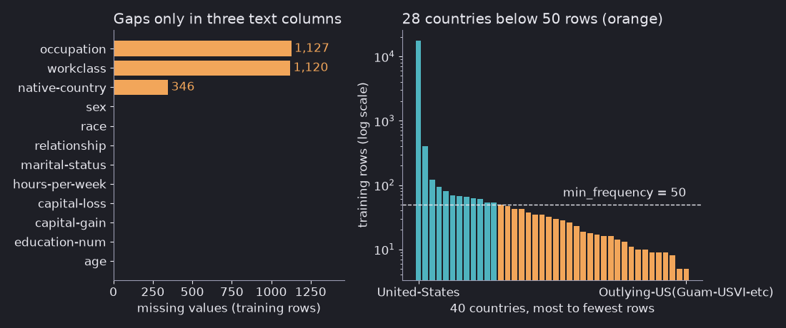
The chart shows the training split from step 4, the rows the pipeline will learn from. Three findings shape the pipeline:
- Only text columns have gaps.
workclass,occupationandnative-countryhave missing values; no numeric column does. We still put an imputer on the numeric columns, because a new row can arrive with a blank number. - 24 rows are exact duplicates. We retain the source records for this preprocessing demonstration. Without person identifiers we cannot tell whether matching rows represent the same person. Duplicate records may cross the split, making evaluation optimistic; their impact was not measured. These are held-out rows, not a demonstrated independent-person benchmark. For a real evaluation, resolve duplicates and grouping before splitting.
- Countries are very uneven. 29,170 rows are United-States, and 20 countries have fewer than 50 rows. Holand-Netherlands has one. A one-hot column learned from one row says almost nothing.
We also drop two columns. fnlwgt is a census sampling weight, not a fact about the person. education is the same information as education-num in text form.
4. Split before any fitting
Split the rows into train (60%), validation (20%) and test (20%), stratified by the label so each part keeps the same share of high earners. This is a static row-split demonstration with the duplicate-record limitation noted above, not proof of generalization to independent people or future years. For time series it would not be: see KFold vs TimeSeriesSplit.
NUMERIC = ["age", "education-num", "capital-gain", "capital-loss", "hours-per-week"]
CATEGORICAL = ["workclass", "marital-status", "occupation", "relationship", "race", "sex",
               "native-country"]
X = df[NUMERIC + CATEGORICAL]
y = (df["income"] == ">50K").astype(int)
X_train, X_rest, y_train, y_rest = train_test_split(
    X, y, test_size=0.4, stratify=y, random_state=SEED)
X_val, X_test, y_val, y_test = train_test_split(
    X_rest, y_rest, test_size=0.5, stratify=y_rest, random_state=SEED)
for name, part, label in [("train", X_train, y_train), ("validation", X_val, y_val),
                          ("test", X_test, y_test)]:
    print(f"{name:10s} {part.shape}  share >50K: {label.mean():.3f}")
train_missing = X_train.isna().sum()
print(train_missing[train_missing > 0].to_string())
print("Train countries with < 50 rows:", (X_train["native-country"].value_counts() < 50).sum())
train      (19536, 12)  share >50K: 0.241
validation (6512, 12)  share >50K: 0.241
test       (6513, 12)  share >50K: 0.241
workclass         1120
occupation        1127
native-country     346
Train countries with < 50 rows: 28
The training split keeps 60% of the rows, so more countries fall under 50 there: 28 of the 40 countries it contains, compared with 20 of 41 in the full file. Holand-Netherlands, the single-row country, landed outside the training split, so the model will never see it.
From here on, every step that learns something (a median, a mean, a category list, model weights) learns it from X_train only. Validation picks a setting. Test is used once, at the end.
5. Measure a baseline first
A model that always predicts the most common class needs no features at all. Its score is the bar the real model has to clear. For more on why this matters, see Start with a baseline.
baseline = DummyClassifier(strategy="most_frequent").fit(X_train, y_train)
print(f"baseline validation accuracy: {accuracy_score(y_val, baseline.predict(X_val)):.3f}")
baseline validation accuracy: 0.759
About three out of four people earn at most $50K, so “always no” is right about three times out of four. That is why accuracy alone can look better than it is; Accuracy is misleading covers this in more detail.
6. Build the ColumnTransformer and the Pipeline
A ColumnTransformer sends each group of columns through its own steps and puts the results side by side:
- Numeric columns: fill gaps with the training median, then standardize.
- Text columns: fill gaps with the word
"missing", then one-hot encode.min_frequency=50merges every category with fewer than 50 training rows into one shared “infrequent” column.handle_unknown="infrequent_if_exist"sends a new category to that column only if that feature has a fitted infrequent group. Otherwise it produces all zeros for the unknown category, as"ignore"does.
Filling with "missing" keeps the fact that a value was blank, so the model can learn from it. The OneHotEncoder docs list the other handle_unknown options. The default, "error", stops on a new category; we test that in step 9.
numeric_steps = Pipeline([
    ("impute", SimpleImputer(strategy="median")),
    ("scale", StandardScaler()),
])
categorical_steps = Pipeline([
    ("impute", SimpleImputer(strategy="constant", fill_value="missing")),
    ("onehot", OneHotEncoder(handle_unknown="infrequent_if_exist", min_frequency=50,
                             sparse_output=False)),
])
preprocess = ColumnTransformer([
    ("num", numeric_steps, NUMERIC),
    ("cat", categorical_steps, CATEGORICAL),
])
model = Pipeline([
    ("preprocess", preprocess),
    ("classify", LogisticRegression(max_iter=1000)),
])
model.fit(X_train, y_train)

features = model.named_steps["preprocess"].get_feature_names_out()
print("Input columns:", X_train.shape[1], "-> model features:", len(features))
print(features[:2].tolist(), "...", features[-2:].tolist())
medians = model.named_steps["preprocess"].named_transformers_["num"].named_steps["impute"].statistics_
print("Learned medians:", dict(zip(NUMERIC, medians.tolist())))
Input columns: 12 -> model features: 62
['num__age', 'num__education-num'] ... ['cat__native-country_missing', 'cat__native-country_infrequent_sklearn']
Learned medians: {'age': 37.0, 'education-num': 10.0, 'capital-gain': 0.0, 'capital-loss': 0.0, 'hours-per-week': 40.0}
Twelve input columns became 62 model features. The last name, native-country_infrequent_sklearn, is the shared column for rare and unseen countries. The medians came from X_train because model.fit received only X_train. When we later call model.predict on validation or test rows, the pipeline only applies those learned values; it does not refit them. That is the leakage protection described in Why fit preprocessing on training data only?.
7. Choose one setting with the validation set
C controls how strongly logistic regression is regularized: a smaller value means a simpler model. Try four values, score each on validation, and keep the best. set_params uses the step name and parameter name joined by two underscores.
val_scores = {}
for C in [0.01, 0.1, 1.0, 10.0]:
    model.set_params(classify__C=C).fit(X_train, y_train)
    val_scores[C] = accuracy_score(y_val, model.predict(X_val))
    print(f"C={C:<5} validation accuracy: {val_scores[C]:.4f}")
best_C = max(val_scores, key=val_scores.get)
model.set_params(classify__C=best_C).fit(X_train, y_train)
print("chosen C:", best_C)
C=0.01  validation accuracy: 0.8444
C=0.1   validation accuracy: 0.8487
C=1.0   validation accuracy: 0.8484
C=10.0  validation accuracy: 0.8495
chosen C: 10.0
All four values land within half a percentage point. C=10 beat C=0.1 by five of the 6,512 validation rows, which is close to noise, and it sits at the edge of the grid. Either would be a reasonable choice; what matters is that the rule (highest validation accuracy) was fixed before looking at the test set. Each fit call refits the whole pipeline, imputers and encoder included, on X_train only.
8. Score the held-out test set once
test_proba = model.predict_proba(X_test)[:, 1]
test_pred = model.predict(X_test)
scores = {
    "baseline_accuracy": accuracy_score(y_test, baseline.predict(X_test)),
    "pipeline_accuracy": accuracy_score(y_test, test_pred),
    "pipeline_roc_auc": roc_auc_score(y_test, test_proba),
}
for name, value in scores.items():
    print(f"{name:18s} {value:.4f}")
baseline_accuracy  0.7591
pipeline_accuracy  0.8471
pipeline_roc_auc   0.9051
| Model, same 6,513 test rows | Accuracy | ROC AUC |
|---|---|---|
| Always predict “<=50K” (baseline) | 0.7591 | 0.5 (no ranking) |
| Pipeline + logistic regression, C=10 | 0.8471 | 0.9051 |
ROC AUC measures how well the predicted probabilities rank high earners above low earners: 0.5 is random, 1.0 is perfect. The pipeline clears the baseline on both measures. This is one split with one seed, and the test set has now been used, so do not go back and tune on it.
9. Predict on raw rows, including an unknown category
New data arrives as raw values, with blanks and new categories. The pipeline needs the same column names, but no manual preprocessing. Here are two made-up applicants who are the same except for the country. The first is from Brazil, which is not in the data at all. The second is from Scotland, which has only a few training rows and so was merged into the infrequent column. Both have a missing workclass and a missing hours-per-week.
Use np.nan for both blanks, matching the CSV loader’s missing-value representation. A default SimpleImputer does not necessarily treat Python None in an object column as np.nan. The assertion below checks that the categorical blank really became "missing", rather than silently taking an unknown-category path.
person = {"age": 45, "workclass": np.nan, "education-num": 13, "marital-status": "Married-civ-spouse",
          "occupation": "Prof-specialty", "relationship": "Husband", "race": "White", "sex": "Male",
          "capital-gain": 0, "capital-loss": 0, "hours-per-week": np.nan}
new_rows = pd.DataFrame([{**person, "native-country": "Brazil"},
                         {**person, "native-country": "Scotland"}])
imputed = model.named_steps["preprocess"].named_transformers_["cat"].named_steps["impute"].transform(new_rows[CATEGORICAL])
assert (imputed[:, CATEGORICAL.index("workclass")] == "missing").all()
print("Training rows: Brazil", (X_train["native-country"] == "Brazil").sum(),
      "| Scotland", (X_train["native-country"] == "Scotland").sum())
print("P(>50K):", model.predict_proba(new_rows)[:, 1].round(4).tolist())
encoded = model.named_steps["preprocess"].transform(new_rows)
print("Same encoded row:", np.array_equal(encoded[0], encoded[1]))
print("Infrequent-country column:", encoded[:, -1].tolist())

strict = OneHotEncoder(sparse_output=False).fit(X_train[["native-country"]].fillna("missing"))
try:
    strict.transform(new_rows[["native-country"]])
except ValueError as error:
    print("Default OneHotEncoder:", error)
Training rows: Brazil 0 | Scotland 9
P(>50K): [0.5043, 0.5043]
Same encoded row: True
Infrequent-country column: [1.0, 1.0]
Default OneHotEncoder: Found unknown categories ['Brazil'] in column 0 during transform
Both rows get the same probability because, after encoding, they are the same row. The model has no column for Brazil; it treats Brazil exactly like Scotland and the other rare countries merged into the infrequent column. The blank workclass became the "missing" category and the blank hours became the training median. With the default encoder, the same input raises a ValueError instead.
That is the honest meaning of “handles unknown categories”: the pipeline does not crash, and nothing more. The prediction for this synthetic Brazilian row rests on the other columns plus whatever the rare-country group taught the model. The test set shows how that group fared:
onehot = model.named_steps["preprocess"].named_transformers_["cat"].named_steps["onehot"]
rare = onehot.infrequent_categories_[CATEGORICAL.index("native-country")]
is_rare = X_test["native-country"].isin(rare).to_numpy()
print("Countries merged into infrequent:", len(rare))
for name, mask in [("rare-country rows", is_rare), ("all other rows", ~is_rare)]:
    print(f"{name:17s} n={mask.sum():5d}  share >50K={y_test[mask].mean():.3f}  "
          f"accuracy={accuracy_score(y_test[mask], test_pred[mask]):.3f}")
Countries merged into infrequent: 28
rare-country rows n=  200  share >50K=0.190  accuracy=0.865
all other rows    n= 6313  share >50K=0.243  accuracy=0.847
The 200 test people from those 28 countries were classified correctly 86.5% of the time, a bit higher than everyone else. Do not read that as “rare countries are handled well”: only 19.0% of them are high earners, so always guessing “<=50K” would already be right for 81.0%. The model adds 5.5 points over that for this group and 9.0 points (75.7% to 84.7%) for the rest. And this group consists of countries the model saw a few times; Brazil had no rows at all. If unseen categories matter in your application, log how often they arrive and measure them once you have labeled examples.
10. Save the fitted pipeline and load it back
Because preprocessing lives inside the pipeline, saving one object saves everything: medians, scaler statistics, category lists and model weights.
joblib.dump(model, OUT / "income_pipeline.joblib")
loaded = joblib.load(OUT / "income_pipeline.joblib")
print("Loaded predictions match:",
      np.array_equal(loaded.predict_proba(X_test), model.predict_proba(X_test)))
pd.DataFrame({"y_true": y_test.to_numpy(), "p_over_50k": test_proba}).to_csv(
    OUT / "test_predictions.csv", index=False)
Loaded predictions match: True
Load the file only with the same scikit-learn version, and only if you trust its source: joblib.load can run code stored in the file. The scikit-learn model persistence guide describes safer formats such as skops and ONNX.
What to try next
Change min_frequency=50 to 10, rerun the steps and check two things first: how many features the encoder now creates, and which countries stay in the infrequent group. Then compare validation accuracy, not test accuracy. The test set above has already been used once. We have not measured this variation, so we make no claim about its effect.
You can also replace LogisticRegression with HistGradientBoostingClassifier and keep the same preprocess object. Step 6 is the part that stays the same when the model changes.
Limits of this run: one random split with seed 0, one dataset from 1994, and a model chosen for clarity rather than best accuracy. The recorded output of the full script is in reference_output.txt.
Implementation references, checked 2026-11-01: ColumnTransformer, SimpleImputer, OneHotEncoder and DummyClassifier.