Time Series Forecasting
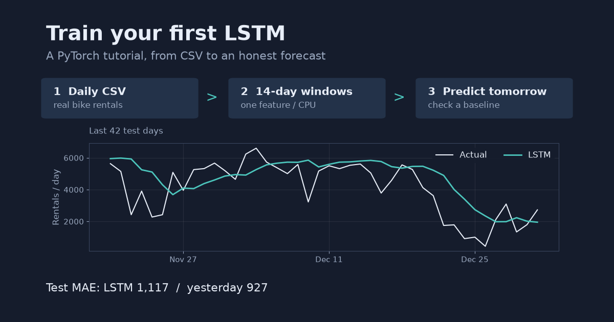
The forecasting posts use the UCI Bike Sharing data (CC BY 4.0) and compare every model with a naive baseline on the same dates. In the next-day LSTM tutorial, yesterday’s count scored a test MAE of 926.6 and the seed-0 LSTM 1,117.2. Results like that are reported as measured.
- Your first LSTM forecast in PyTorch: from CSV to predictions
A step-by-step LSTM tutorial using real daily bike rentals: load and plot a CSV, build 3D input windows, train on CPU, and compare next-day predictions with yesterday's value. Complete runnable Python code included.
- Recursive vs direct multi-step forecasting: what a one-step score hides
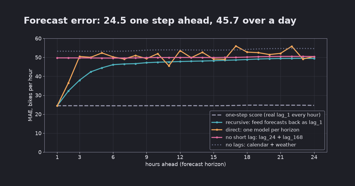
A model with lag features scored MAE 24.5 one hour ahead. Forecasting the next 24 hours, the same model averaged 45.7. Recursive, direct and "no short lag" strategies compared on real hourly data with scikit-learn, with code.
- KFold vs TimeSeriesSplit: how shuffled cross-validation hides time-series leakage
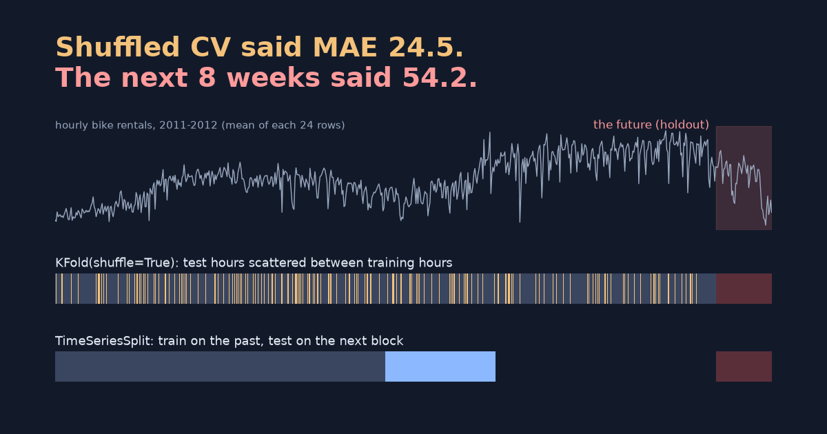
On two years of hourly bike rentals, shuffled KFold estimated MAE 24.5 while the next 8 weeks gave 54.2. When TimeSeriesSplit helps, why lag features change the picture, and the rolling-feature leak no split can catch.
- LSTM input shape explained: (batch, timesteps, features)
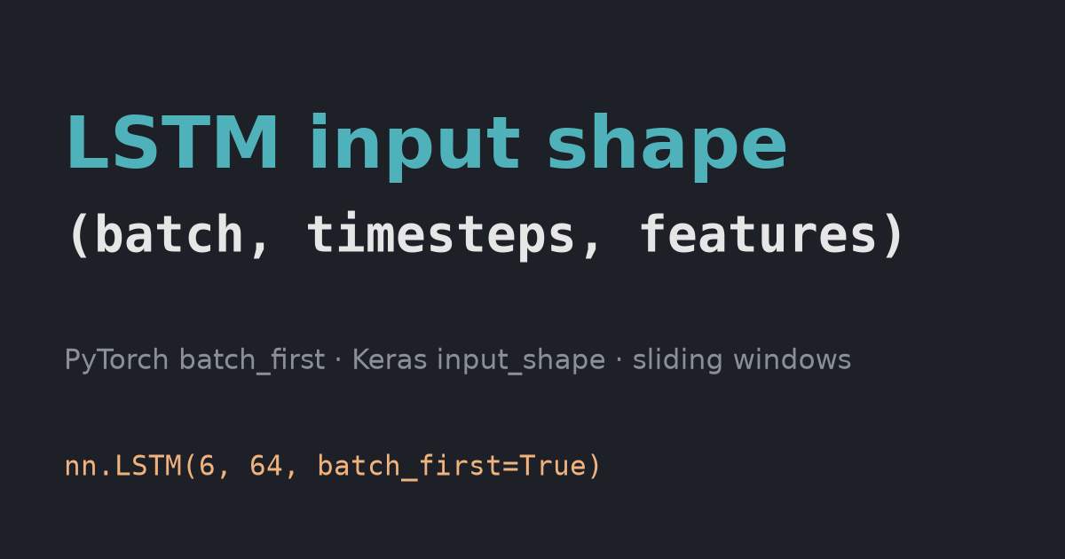
What each of the three LSTM input dimensions means, how to build them from a time series with sliding windows, and the PyTorch batch_first default that silently mixes your samples. Tested with PyTorch 2.14 and Keras 3.15.